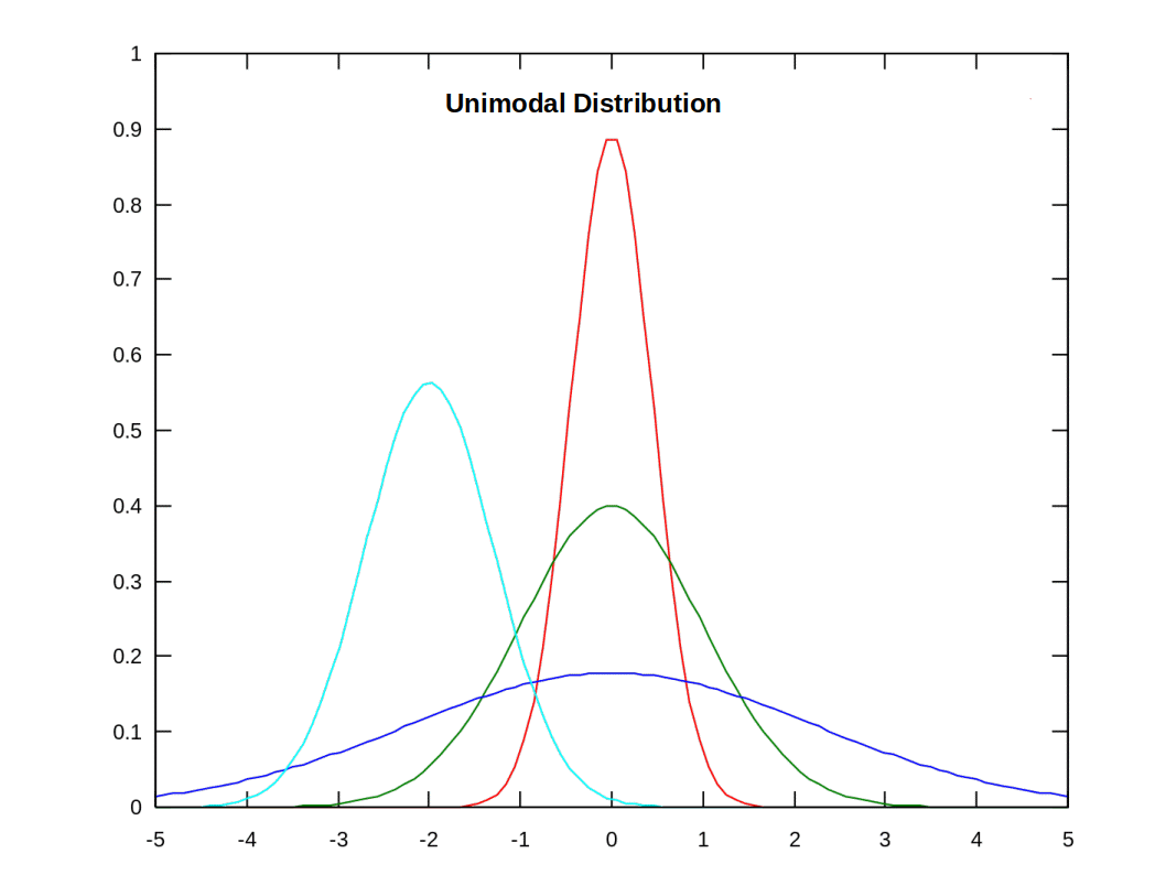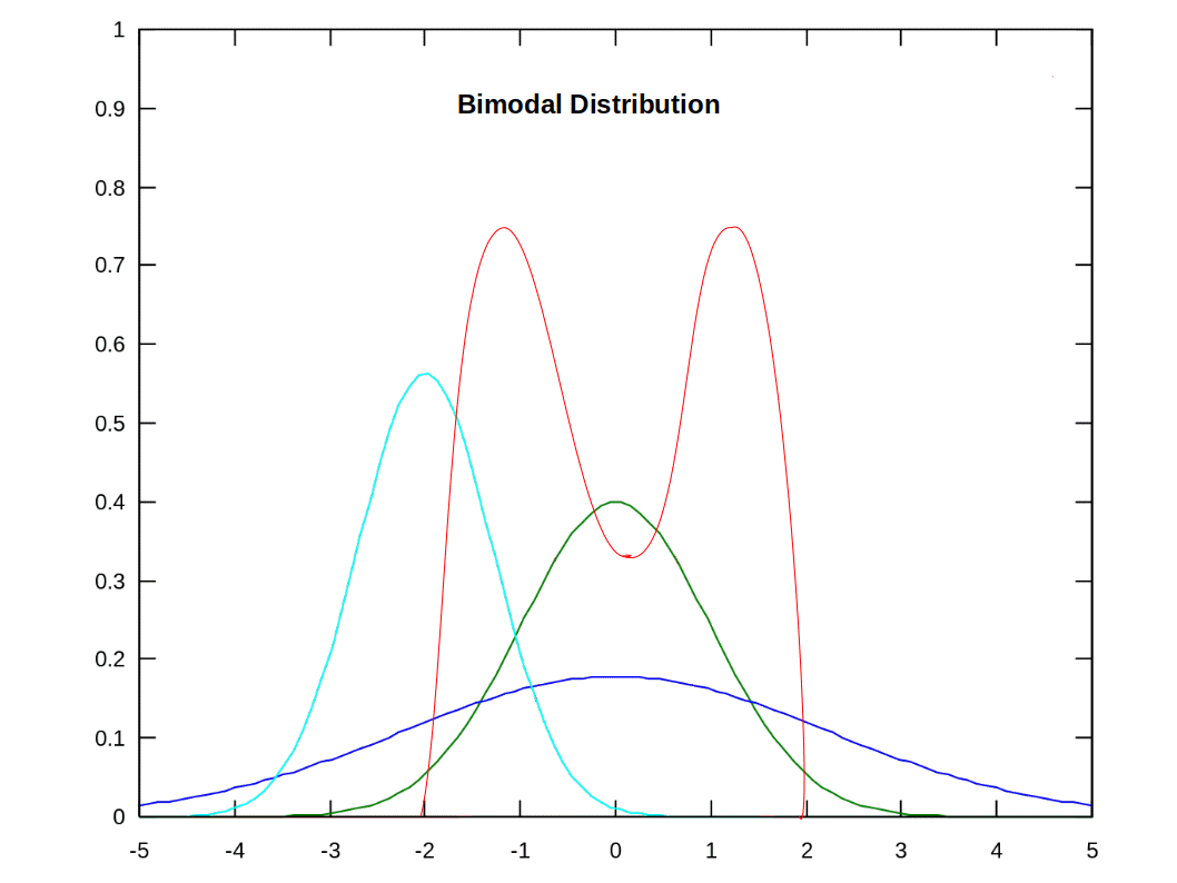
 Like, Arithmetic Mean and Median, Mode is also a measure of central tendency. It is most common item of a series. It represents the most typical value of a series. It is the value which occurs the largest number of times in a series. Mode is the value around which there is the greatest concentration of values. In other words, it is the item having the largest frequency. In some cases, there may be more than one point of concentration of values and the series may be bi-modal or multi-modal. When one value occurs more frequently than any other value, the distribution is called unimodal.
 The word mode is derived from the French word ‘la mode’ which means fashion or the most popular phenomenon. Mode, is thus the most popular item of a series around around which there is the highest frequency density. It is denoted by Mo.
There can be more than one mode in a distribution. A distribution with a single modal value is called Unimodal.
 A distribution with two model value is called Bimodal and with more than two is Multimodal.
 It may so happen that there may be no mode at all in a distribution when no value appears more frequently than any other value. For example, in a series 1, 1, 2, 2, 3, 3, 4, 4, there is no mode.
Let us discuss the methods of finding mode in diffrent series of data.
INDIVIDUAL SERIES
Comparing to mean and median, computation of mode is easy. In individual series, mode is that value which repeats highest number of times. It is often found by mere inspection.
Here the item 2 repeats two times; 5 repeats four times and 7 repeats two times. All the other items occurs once. So the most frequent item is 5; and therefore the mode is 5.
Here the item 2 repeats two times; 5 repeats four times; 7 repeats two times and 3 repeats four times. All the other items occur once. When there are two or more values having the same maximum frequency, mode is said to be ill-defined. We cannot find the modal value of this series in the said way. In such case; we use a formula for finding mode, which is known as the empirical formula.
Mode = 3 median - 2 mean
Here, Mean = \( {{{\frac{N}{2}} }} \)
= \( {{{\frac{2+5+7+3+6+4+3+5+8+2+3+7+5+10+5+9+3}{17}} }} \)
= \( {{{\frac{87}{17}} }} \)
= 5.1
In order to find median we need to arrange the data in ascending order.
2, 2, 3, 3, 3, 3, 4, 5,5, 5, 5, 6, 7, 7, 8, 9, 10
Median = value of the \( \Biggl[{{{\frac{N+1}{2}} }}\Biggl]^{th} \) item
= \( \Biggl[{{{\frac{17+1}{2}} }}\Biggl]^{th} \) item
= value of the 9th item
= 5
∴ Mode = 3 median - 2 mean
= (3 × 5) - (2 × 5.1)
= 15 - 10.2
= 4.8
DISCRETE SERIES
In discrete series, mode is determined just by inspection. The item having highest frequency is taken as mode.
| X | Frequencies |
|---|---|
| 5 | 7 |
| 10 | 12 |
| 15 | 15 |
| 20 | 18 |
| 25 | 13 |
| 30 | 10 |
| 35 | 5 |
| 40 | 2 |
The value having highest frequency is 20; and therefore, 20 is the modal value.
CONTINUOUS SERIES
I n continuous series, mode lies in the class having highest frequency. Hence the modal class may be determined either by inspection or by grouping table. Then mode is determined using the formula:
 L = lower limit of the modal class
D1 = difference between the frequencies of the modal class and the class preceding it (ignoring the sign)
D2 = difference between frequencies of the modal class and the class succeeding it (ignoring the sign); and
h = class interval of the modal class
| X | Frequencies |
|---|---|
| 0 - 5 | 7 |
| 5 - 10 | 10 |
| 10 - 15 | 12 |
| 15 - 20 | 18 |
| 20 - 25 | 13 |
| 25 - 30 | 8 |
| 30 - 35 | 5 |
| 35 - 40 | 2 |
The class having highest frequency is 15 - 20
∴ Modal class = 15 - 20
Now, mark the modal class. Then mark frequencies just above and below the modal class.
| X | Frequencies |
|---|---|
| 0 - 5 | 7 |
| 5 - 10 | 10 |
| 10 - 15 | 12 |
| 15 - 20 | 18 |
| 20 - 25 | 13 |
| 25 - 30 | 8 |
| 30 - 35 | 5 |
| 35 - 40 | 2 |
L = 15, D1 = 18 - 12 = 6, D2 = 18 - 13 = 5, h = 5
\( M_o \,= \,{ L + \frac{{D_1}}{{D_1}+{D_2}} × h} \)
\( = \,{ 15 + \frac{{6}}{{6}+{5}} × 5} \)
\( = \,{ 15 + \frac{{30}}{{11}}} \)
= 15 + 2.73
= 17.73
INCLUSIVE CLASS
| X | Frequencies |
|---|---|
| 0 - 9 | 22 |
| 10 - 19 | 34 |
| 20 - 29 | 53 |
| 30 - 39 | 85 |
| 40 - 49 | 48 |
| 50 - 59 | 26 |
| 60 - 69 | 18 |
| 70 - 79 | 14 |
We need to convert the classes into the exclusive form as in the given below table.
| X | Frequencies |
|---|---|
| .5 - 9.5 | 22 |
| 9.5 - 19.5 | 34 |
| 19.5 - 29.5 | 53 |
| 29.5 - 39.5 | 85 |
| 39.5 - 49.5 | 48 |
| 49.5 - 59.5 | 26 |
| 59.5 - 69.5 | 18 |
| 69.5 - 79.5 | 14 |
The class having highest frequency is 29.5 - 39.5
∴ Modal class = 29.5 - 39.5
Now, mark the modal class. Then mark frequencies just above and below the modal class.
L = 29.5, D1 = 85 - 53 = 32, D2 = 85 - 48 = 37, h = 10
\( M_o \,= \,{ L + \frac{{D_1}}{{D_1}+{D_2}} × h} \)
\( = \,{ 29.5 + \frac{{32}}{{32}+{37}} × 10} \)
\( = \,{ 29.5 + \frac{{320}}{{69}}} \)
= 29.5 + 4.64
= 34.14
OPEN END CLASSES
| X | Frequencies |
|---|---|
| Less than 100 | 40 |
| 100 - 200 | 89 |
| 200 - 300 | 148 |
| 300 - 400 | 64 |
| 400 and above | 39 |
In the above given distribution, the first and last classes are open end classes. But as in the calculation of AM, it is not needed to make assumptions about their class intervals . We may just leave them as they are.
Let us create a table to show model classes, lower and upper frequencies of model class frequency.
| X | Frequencies |
|---|---|
| Less than 100 | 40 |
| 100 - 200 | 89 |
| 200 - 300 | 148 |
| 300 - 400 | 64 |
| 400 and above | 39 |
The class having highest frequency is 200 - 300
∴ Modal class = 200 - 300
Now, mark the modal class. Then mark frequencies just above and below the modal class.
L = 200, D1 = 148 - 89 = 59, D2 = 148 - 64 = 84, h = 100
\( M_o \,= \,{ L + \frac{{D_1}}{{D_1}+{D_2}} × h} \)
\( = \,{ 200 + \frac{{59}}{{59}+{84}} × 100} \)
\( = \,{ 200 + \frac{{5900}}{{143}}} \)
= 200 + 41.25
= 241.3
LESS THAN CUMULATIVE FREQUENCY
| Value | Frequencies |
|---|---|
| Less than 60 | 65 |
| " " 80 | 185 |
| " " 100 | 270 |
| " " 120 | 342 |
| Less than 140 | 400 |
In the above given distribution, only cumulative frequencies are given. We have to find class and simple frequencies of each class. This is shown in the below given table.
| Value | Frequencies |
|---|---|
| 40 - 60 | 65 |
| 60 - 80 | 120 |
| 80 - 100 | 85 |
| 100 - 120 | 72 |
| 120 - 140 | 58 |
The class having highest frequency is 60 - 80
∴ Modal class = 60 - 80
Now, mark the modal class. Then mark frequencies just above and below the modal class.
L = 60, D1 = 120 - 65 = 55, D2 = 120 - 85 = 35, h = 20
\( M_o \,= \,{ L + \frac{{D_1}}{{D_1}+{D_2}} × h} \)
\( = \,{ 60 + \frac{{55}}{{55}+{35}} × 20} \)
\( = \,{ 60 + \frac{{1100}}{{90}}} \)
= 60 + 12.2
= 72.22
WITH UNEQUAL CLASS INTERVALS
| Value | Frequencies |
|---|---|
| 0 - 30 | 9 |
| 30 - 40 | 8 |
| 40 - 50 | 15 |
| 50 - 60 | 9 |
| 60 - 70 | 3 |
| 70 - 90 | 4 |
In the above given distribution the class intervals are unequal. For finding mode, the frequencies should be adjusted to make the class intervals equal, Smallest class interval is 10. So make all the classes with class interval 10. Class 0-30 to be replaced by classes 0-10, 10-20 and 20-30 and the class 70-90 to be replaced by classes 70-80 and 80-90. The frequencies of the classes 0-10, 10-20 and 20-30 will be \( { \frac{{9}}{{3}}} = 3 \) each; and frequencies of the classes 70 - 80 and 80 - 90 will be \( { \frac{{4}}{{2}}} = 2 \).
We can create a table showing adjusted classes and frequencies in the below given table.
| Value | Frequencies |
|---|---|
| 0 - 10 | 3 |
| 10 - 20 | 3 |
| 20 - 30 | 3 |
| 30 - 40 | 8 |
| 40 - 50 | 15 |
| 50 - 60 | 9 |
| 60 - 70 | 3 |
| 70 - 90 | 4 |
| 70 - 80 | 2 |
| 80 - 90 | 2 |
The class having highest frequency is 40 - 50
∴ Modal class = 40 - 50
Now, mark the modal class. Then mark frequencies just above and below the modal class.
L = 40, D1 = 15 - 8 = 7, D2 = 15 - 9 = 6, h = 10
\( M_o \,= \,{ L + \frac{{D_1}}{{D_1}+{D_2}} × h} \)
\( = \,{ 40 + \frac{{7}}{{7}+{6}} × 10} \)
\( = \,{ 40 + \frac{{70}}{{13}}} \)
= 40 + 5.38
= 45.38
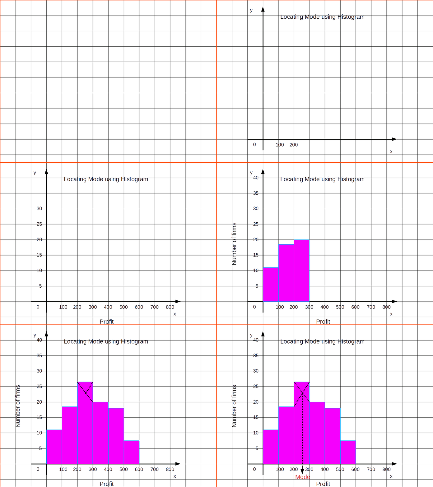
LOCATING MODE GRAPHICALLY
STEPS
- Draw a histogram of the given data.
- Draw two lines diagonally in the inside of the modal class bar, starting from each corner of the bar to the upper corner of the adjacent bar.
- Then, draw a perpendicular line from the point of intersection to the X - axis, which gives us-the modal value.
| X | Frequencies |
|---|---|
| 0 - 100 | 12 |
| 100 - 200 | 18 |
| 200 - 300 | 27 |
| 300 - 400 | 20 |
| 400 - 500 | 17 |
| 500 - 600 | 6 |
Let us find mode by drawing histogram for the above given distribution.


MERITS OF MODE
- Mode is the true representative value of a distribution.
- It is not affected by extreme items.
- It can be determined in open-end distributions.
- It can be used to describe qualitative phenomenon.
- It can also be determined graphically.
DEMERITS OF MODE
- In the case of bi-modal series, mode cannot be determined.
- It is not capable of algebraic treatment.
- It is not based on each and every item of the series.
- It is not a rigidly defined one.
Relative Position of Arithmetic Mean, Median and Mode
$$ Mode > Median >Mean $$
$$or$$ $$ Mode < Median < Mean $$
Median is always in between Mode and Mean.
karl Pearson has expressed a relationship for a moderately skewed distribution as follows:
$$ Mode = 3 Median - 2 Mean $$


