
Demand A consumer’s desire to buy a good is usually considered as demand. But in economics mere desire does not become demand. The consumer should have the ability and willingness to buy along with his desire for a good. Therefore, Demand-is desire backed by willingness to pay and ability to pay.
Demand for a Commodity Demand for a commodity is the quantity of a commodity that a consumer is willing to buy in a given period of time at a given price.
The quantity of the good a consumer decides to buy depends on the price of the good, the prices of other goods, the income of the consumer and the taste and preferences of the consumer. The demand is a multivariate relationship. It is determined by various factors simultaneously. When changes occur in the factors or determinants change also takes place in the quantity of the good he decides to buy.
Individual Demand Individual demand can be defined as the quantity of a commodity that an individual consumer is willing to buy from the market in a given period of time at a given price.
Household Demand Household demand can be defined as the quantity of a commodity that a household is willing to buy from the market in a given period of time at a given price.
Demand Function The functional relationship between demand and the determinants of demand is called Demand Function, i.e., the relationship between demand (q) and its determinants such as price of the commodity (P), Income of the consumer (M), Prices of related commodities (Pr) and Taste and preference of the consumer (T).
$$ \mathbf{Algebraically, q = f(P, Pr, M, T)} $$
The price, P is the most important factor among the determinants of demand. Therefore, the consumer’s demand for a commodity can be written as the function of price.
$$ \mathbf{q \,=\, d(P)} $$
Law of Demand The consumer’s demand for a commodity and its price have a negative or inverse relationship. Other things remaining unchanged, the inverse relationship between demand and price of the commodity is called law of demand. That is, as the price of the commodity falls the quantity demanded rises and as the price rises quantity demanded falls, other things remaining unchanged. The Law of Demand is based on the assumption that the consumer’s income, prices of related commodities, tastes and preferences of the consumer are constant.
Demand Curve The graph which shows the inverse relationship between demandand price is called Demand Curve. In other words, the graphical representation of the demand function is called the demand curve. Below Diagram shows a demand curve.
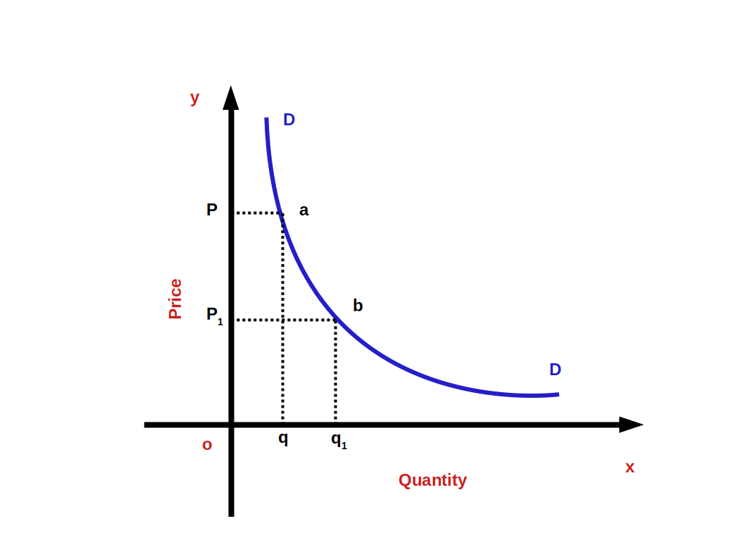
Quantity is represented along x-axis and price is represented along y-axis. DD is demand curve. This curve shows the inverse relationship between price and demand. When price rises from OP1 to OP quantity demanded falls from Oq1 to Oq. When price falls from OP to OP1 quantity demanded rises from Oq to Oq1. So the curve DD shows the inverse relationship between price and demand. That is why the demand curve is sloping downward from left top to right bottom. The slope of demand curve is negative.
Why does demand rise when price falls? Substitution effect and income effect are the two main reasons for the inverse relationship between price and quantity demanded. The sum of substitution effect and income effect is price effect.
Price effect:
Change in demand caused by change in price is called price effect. Price effect can be divided into two: substitution effect and income effect.
Substitution effect:
Substitution effect considers two commodities When there is a fall in the price of one of them; there is a change in relative price. As a result more of the cheaper good is demanded instead of the good with unchanged price. The cheaper good is substituted in the place of the costlier good.
Income effect:
Income effect is the change in the demand of a commodity due to the change in real income of the-consumer. When price of a commodity goes down, purchasing power increases. This is an increase in real income. As a result, the consumer demands more of it.
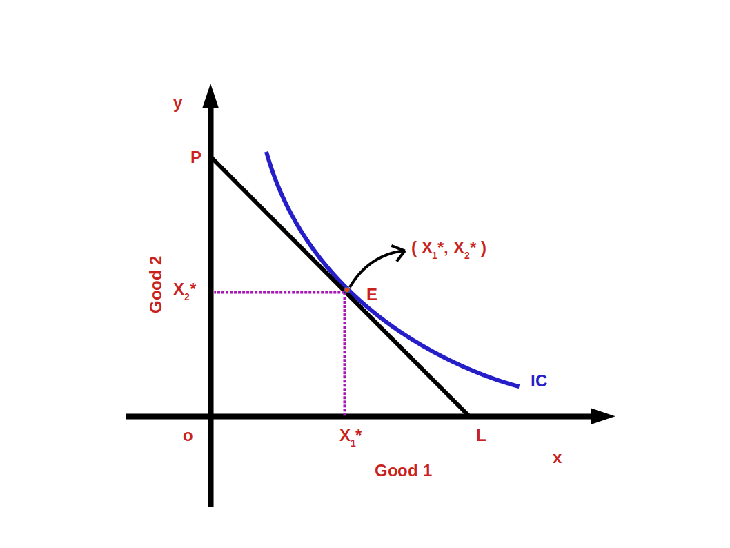
Look at the above diagram. Here on the budget line PL at point E the consumer is in equilibrium State. The budget line PL touches the indifference curve IC at point E.
The Consumer’s equilibrium bundle is (x1*, x2*). The cost of this bundle is P1x1* + P2x2* = M, When the price of one commodity falls two changes take place:
Suppose the price of good 1 falls
- The price of good 1 falls when compared good 2. That is relative price falls. This makes the consumer capable of buying more units of the less expensive good.
- As his purchasing power has increased, the consumer’s real income increases. This enables the consumer to buy the same quantity of goods before price fall for a lesser price.
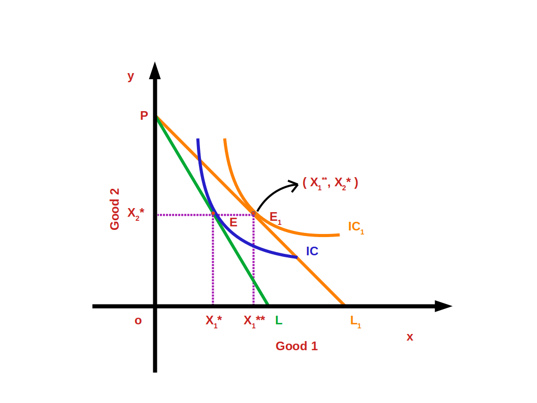
Look at the above diagram. The price of good 1 has fallen. As a result the budget line PL has changed to PL1. The indifference curve IC1 touches the budget line PL1, at point E1. At point E1 the consumer accepts the bundle (x1**, x2*) and he is in equilibrium stage. Bundle E (x1*, x2*) changes to the new bundle E1 (x1**, x2*). This change from E to the new bundle E1 (x1**, x2*) is called price effect.
As a result of fall in price of good 1 the measure of demand for good 1 increases from x1* to x1** . The change in the demand of good due to change in price is called price effect. Price effect is the combination of substitution effect and income effect. Price effect can be divided into substitution effect and income effect. To separate substitution effect and income effect we have to remove the gain in real income due to price fall. That is to say, to separate price effect into substitution effect and income effect we have to bring about a change in the expense that would enable him to select the bundle before price change.
Suppose the price of good 1 changes from P1 to ΔP1
Now the new price of good 1 is P1 - ΔP1. The price of good 2 remains unchanged as P2.
The price of the bundle ( x1*, x2* ) would be
= ( P1 - ΔP1)x1* + P2x2*
= P1x1* - ΔP1x1* + P2x2*
= P1x1* + P2x2* - ΔP1x1*
= M - ΔP1x1* ( P1x1* + P2x2* = M )
So there is a decrease in the income of the consumer ΔP1x1*. The difference in expense would be ΔP1x1*.
i.e. change in expenses before and after change in price would be ΔP1x1*.
Price fall of good 1 causes gain in income. To counter this gain in income, expenses are to be changed. Change in expense in (ΔP1x1*.). This is to be subtracted from the consumer’s income.
$$ {i.e,\, (M-ΔP_1{x_1^*} )} $$
In the below diagram the budget line changes to P'L’. The budget line P'L' passes towards the left through the bundle E and parallel to the budgetline PL1.

Now the consumer has adjusted his income equal to his previous purchasing power. The change from point E to point E2 is called substitution effect. Demand for good 2 is decreased from x2* to x2' at point E2. Thus the means of good 1 increase from x1* to x1' . In the place of bundle (x1*, x2*) bundle (x1', x2' ) is substituted. More of the cheap good is substituted in the place of goods with unchanged price. This is known as Substitution Effect.
The change from point E2 to point E1 is called Income Effect. He changes from the bundle ( x1', x2' ) to the bundle ( x1**, x2* ). When there is a change in the price of good 1 there is a corresponding change in the purchasing power. This causes changes in measure of demand, and is called income effect.
Total effect is the change from E to E1 . It is the sum of substitution effect and income effect.
$$ {i.e,\,PE \,=\, SE \, + \, IE} $$
Therefore there exists an inverse relationship. These two affects, the amount of demand and its price.
Let us explain these effects using numerical data. Suppose a consumer’s income is ₹30.
Price of good 1 = ₹10
Price of good 2 = ₹5
The consumer’s most preferred bundle is (2, 2). In the below graph, the most preferred bundle (2, 2) is marked in the budget line 10x1 + 5x2 = 30.
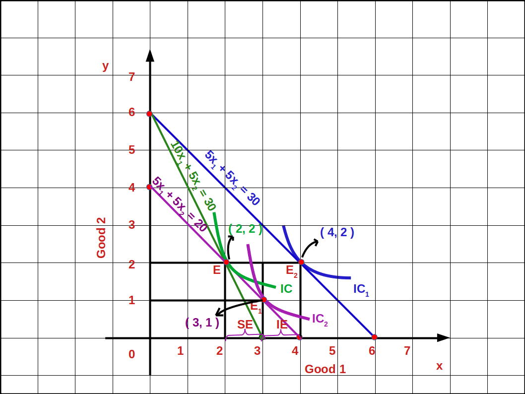
Now let us suppose that the price of good 1 falls from ₹10 to ₹5. The relative price also comes down. Now the budget line is 5x1 + 5x2 = 30 and the consumer's most preferred bundle is (4, 2).
The change from bundle (2, 2) to the bundle (4, 2) is called price effect. That is, as the price of good 1 decreased the consumer can buy 4 units of it instead of 2 units, More than that, because of price fall, the consumer can buy the first bundle (2, 2) for ₹20. This is income effect.
₹5×2 + ₹5×2 = ₹10 + ₹10 = ₹20
If the consumer’s income comes down by ₹10 (₹30 - ₹20 = ₹10) he can manage to buy the bundle (2, 2). Then the budget line would become 5x1 +5x2 = 20. This budget line moves towards the left and goes parallel to the budget line. 5x1 +5x2 = 30. Now the consumer gets an additional income of ₹10. With this money he can buy more units of the good, if he wants. If he wants to buy more of good 1 he will be able to buy 5x1 = 10.
\( x_1\,=\,{\frac{10}{5}}\,=\,2 \) (two units).
If he wants to buy more of good 2 he can buy 5x2 = 10.
\( x_2\,=\,{\frac{10}{5}}\,=\,2 \) (two units).
Or he can buy one unit extra each of good 1 and good 2.
So, when price falls due to substitution effect and income effect, its demand increases. That’s why the demand curve has a negative slope.
When measure of good 1 increases from 2 units to 4 units it is price effect. When the measure of good 1 increases from unit 2 to unit 3 it is substitution effect.
When the measure of good 1 increases from 3 to 4 units it is income effect.
Linear Demand The relation between demand and price can be linear or non linear. A linear demand curve can be algebraically written as
$$ {q\,=\,a\,-\,bP\,;\,0≤P≤ {\frac{a}{b}}} $$
$$ {=\,0\,;\,P > {\frac{a}{b}}} $$
In this linear demand equation
a is vertical intercept
-b is the slope of the demand curve
P is price of good
q is quantity demanded
Moreover,
$$ {If\, price\, =\, 0} $$
$$ {demand \,will \,be \,=\,a} $$
$$ {If\, price\, is \,=\,{\frac{a}{b}}}$$
$$ {demand \,will \,be \,=\,0} $$
Look at the below diagram.
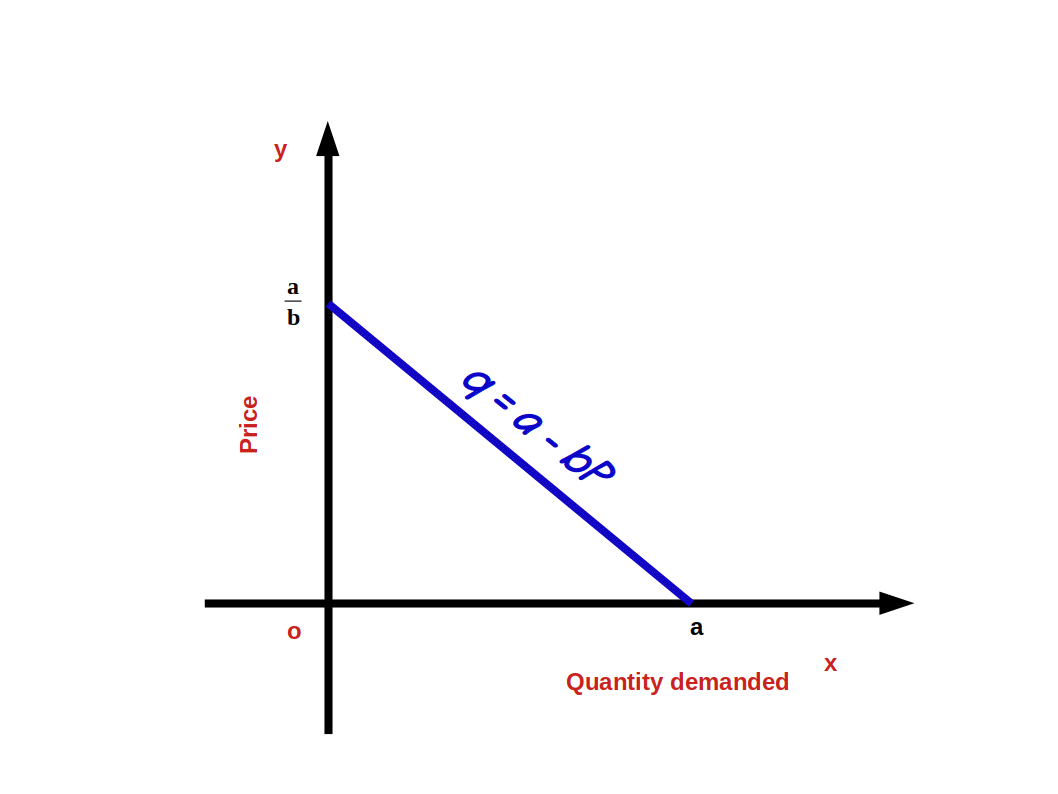
Linear demand curve is shown in the above given diagram. The slope of the demand curve indicates the rate of change in demand according to change in price. That means, whenever there is a change of one unit in price, demand changes by —b unit. Since b is negative the relation between demand and price will be inverse. If price rises by 1 unit, demand will fall by —b unit. Since b is negative the relation between demand and price will be inverse. Price increase by one unit brings down demand by b unit.
$$ {Demand \,curve \,slope\,{\frac{Δq}{ΔP}}\,=\,-\,b}$$
In the law of demand equation we can give values to a and b and the demand curve. Suppose
a = 10
b = 2
Then we get the demand equation
$$ {\,q \,=\,10\,-\,2P} $$
Here 0 ≤ P ≤ 5
If P > 5 demand will be 0
When P = 0, q = 10
i.e. q= 10 - 2 x 0 = 10 - 0 = 10
This is the horizontal intersect. If demand is 0 price would be 5.
0 = 10 - 2P (q = 0)
2P = 10
P = \({\frac{10}{2}} \) = 5, This is Vertical intercept.
Below given graph gives linear demand curve.

Using the law of demand equation q = 10 - 2P, we can find the different values of demand when price changes from 0 to 5, This is given in table 2.7.
| Table 2.7 | |||
| Price (P) | Demand (q) | Method of calculation. q = 10 - 2P | |
|---|---|---|---|
| 0 | 10 | q = 10 - 2 × 0 = 10 - 0 = 10 | |
| 1 | 8 | q = 10 - 2 × 1 = 10 - 2 = 8 | |
| 2 | 6 | q = 10 - 2 × 2 = 10 - 4 = 6 | |
| 3 | 4 | q = 10 - 2 × 3 = 10 - 6 = 4 | |
| 4 | 2 | q = 10 - 2 × 4 = 10 - 8 = 2 | |
| 5 | 0 | q = 10 - 2 × 5 = 10 - 10 = 0 | |
The table showing the relations between a consumer’s demand and price is called individual demand schedule.
Factors determining demand for a commodity or determinants of demand.
As per conventional principle of demand, demand for a commodity is determined mainly by four factors - price, income, price of other commodities and the consumer’s tastes and preferences. We shall now see how these factors affect demand.
Price of a commodity or own Price
The most important factor that determines demand for a commodity is its price. There is an inverse relation between the price and demand of a commodity. That is, when price increases demand decreases; when price decreases demand increases. This is very clear from the law of demand.Income of the consumer
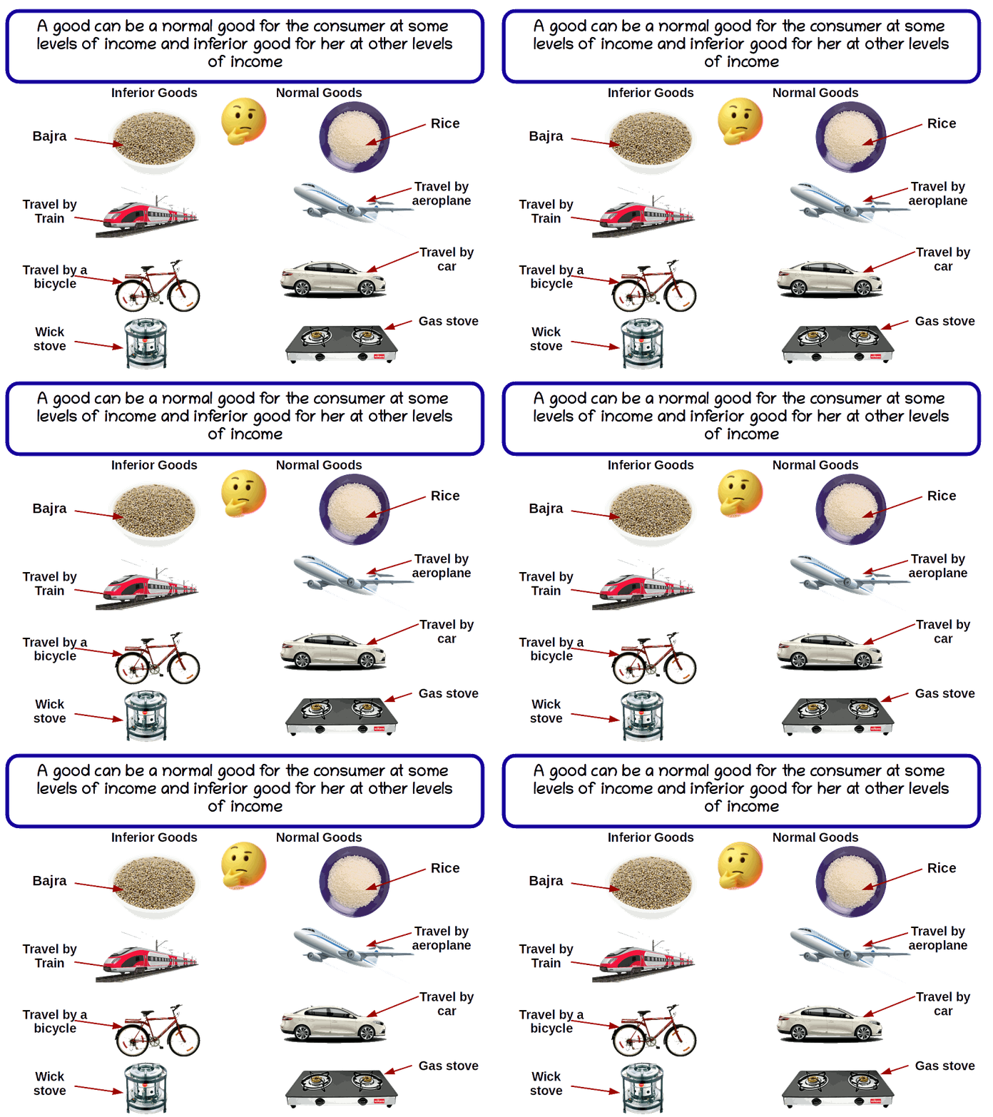
Another’ factor that determines demand is the consumer’s income. The relation between income and demand depends on the nature of goods. Based on income we can divide goods into normal goods and inferior goods.- Normal goods: When the consumer’s income increases demand for the goods increases; when his income decreases demand also decreases. Such goods are called normal goods.
- Inferior goods: When the consumer’s income increases, demand decreases; when his income decreases demand increases. These goods are called inferior goods. The relation between Demand for such goods and the consumer’s income is inverse.
Prices of other related goods
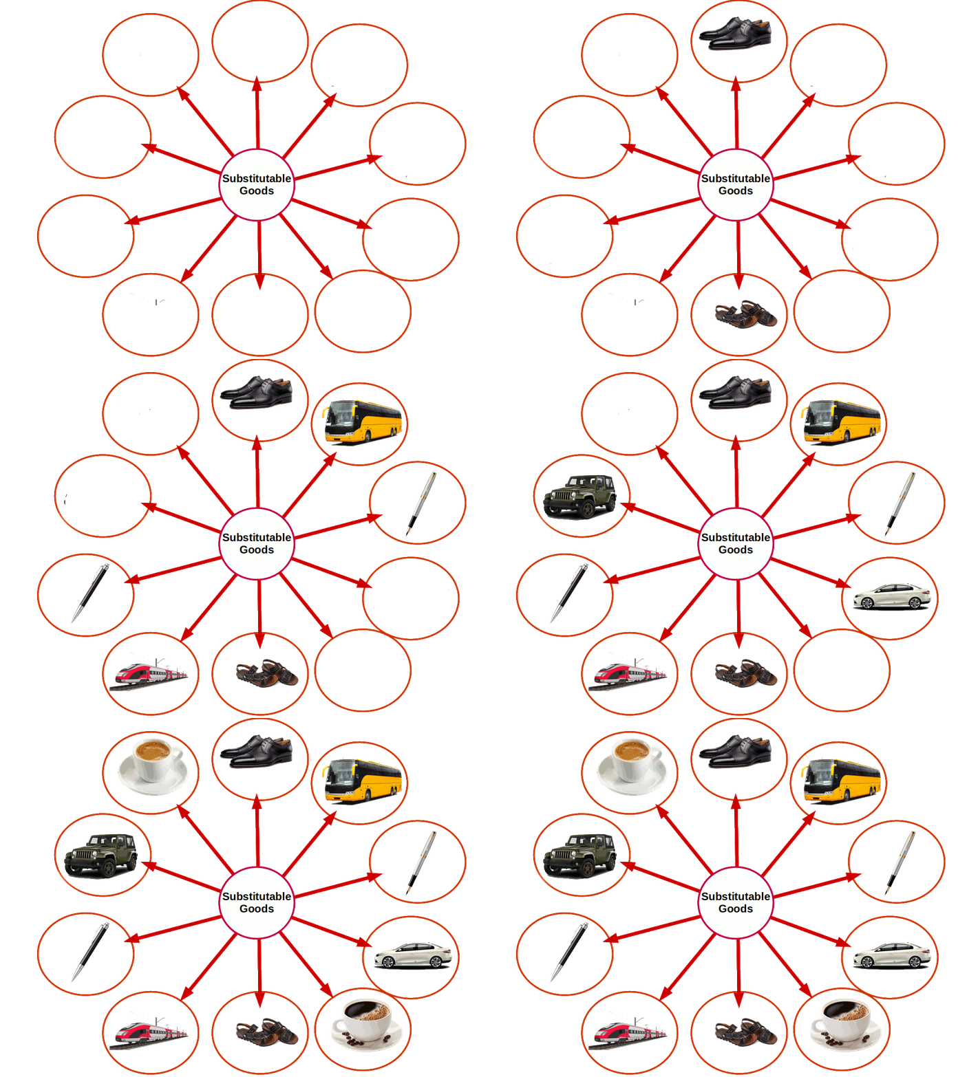
The price of other related goods is another factor that determines the demand for a commodity. On the basis of the relation between its price and demand goods can be classified under two heads-- Substitute goods: Goods that are used as substitutes to satisfy a need are called substitute goods.
- Complementary goods: When more than one good are required to satisfy a want, such goods are called complementary goods.
Taste and preferences
Another factor that determine price is the taste and preferences. When the taste of a consumer for a particular good increases, demand for that good also increases, when his taste for such goods decreases demand for that good also decreases.
Goods like TV, computer, good clothes etc. are normal goods for one person; to another person, these things may not be normal goods, Relation between the consumer's income and his demand for normal goods is positive. i.e.,consumer’s income and demand for mormal goods move in the same direction.
Kerosene stove is inferior to gas stove. Bus travel is inferior to travel by car. Cheap food grains is inferior to rice.
(a) Substitute goods
(b) Complementary goods.
Coffee and tea, bus and train, car and jeep, shoes and slippers are examples for substitute goods. Relation between price of substitute goods and demand is positive. On two substitute goods the price of one will change in the same direction as the demand for the other. When price of tea increases, demand for coffee increases; when price of tea decreases demand for coffee also comes down.
Pen and ink, car and petrol / diesel, lock and key and shoes and socks are complementary goods. The relation between price and demand of comple- mentary goods is inverse. They move in opposite directions. That is, when the price of one complementary good increases the demand for the other decreases. When price decreases demand increases.

Changes in Demand Changes in demand can be generally divided into two:
1. Movement along the demand curve
2. Shift of the demand curve
Movement along the demand curve
Change in demand due to change in price is called movement along the demand curve. Change occurs in the demand ‘curve because of the change in the price of the commodity. No change takes place in non-price factors like the consumer's income. Price of other related goods, consumers tastes and preferences. Change along the demand curve can be of two types-Shift of Demand Curve
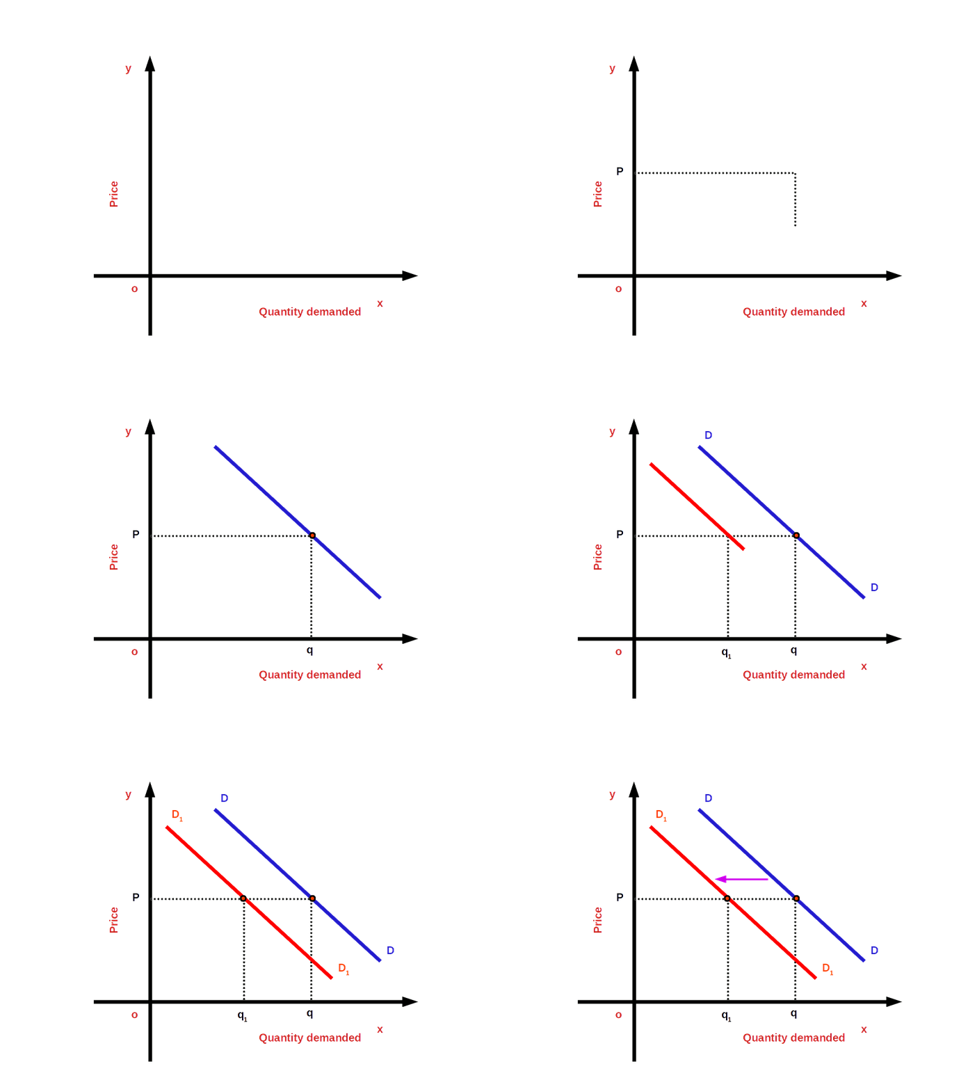
Change in the demand for commodity caused by changes in non-price factors is called shift of Demand Curve. Changes in factors other than price cause shift in the demand curve, For example, change in income. Shift of demand curve can be of two types:
(a) Expansion of demand
(b) Contraction of demand
Expansion of demand:
Downward movement along the demand curve due to fall in price is called expansion of demand. Increase in demand due to price decrease is called expansion of demand.
Look at the below given diagram. When the price of the commodity goes down from P to P1 demand increases from q to q1. In the demand curve, DD, there is a change from point ‘a’ to point ‘b’. This change from a to b is expansion of demand.

Contraction of Demand:
Upward movement along the demand curve due to price rise is called contraction of demand. In other words, when price of a commodity increases due to a fall in demand we call it contraction of demand.
In the below diagram, the price of a commodity increases from P1 to P. And demand for the commodity decreased from q1 to q. On the demand curve DD from point there is a shift from point b to point a. This change from point b to point a is called contraction of demand.

(a) increase in demand
(b) decrease in demand
Increase in demand:
Rightward or upward shift of the demand curve due to favourable changes in non-price factors is called increase in demand. In other words, when more quantity is demanded at a given price or the same price is known as increase in demand. Look at the below given diagram. There DD is the first demand curve. There is a demand for good Og at price OP. As a result of favourable changes in non-price factors DD changes to the new demand curve D1 D1 and goes towards the right. Then demand increases from Oq to Oq1 . The price continues the same OP. The change towards the right of demand curve DD to D1 D1 is called demand increase.

Decrease in demand:
On account of unfavourable changes in non-price factors the demand curve changes towards the left or downward. This change of the demand curve is called decrease in demand. That means, when less quantity is demanded at the given price or the same price, we have decrease in demand. In the below given diagram DD is the first demand curve. At price OP, Oq goods are demanded . On account of unfavourable changes in non price factors the demand curve DD changed towards the left to the new demand curve D1D 1. Then demand decreases from Oq to Oq1. But the price OP remains unchanged . Decrease in demand is then , the change towards the left of demand curve DD to D1D1.
Market Demand Market Demand is the quantity of a commodity that all consumers in a market are willing to buy at different prices at a fixed or given time. This is the total of individual demands. This is done by adding up horizontally all the individual demand tables. Look at the table 2.8. It icludes two individual demand and market demnad.
| Table 2.8 Market Demand | |||||
|---|---|---|---|---|---|
| Indiidual A | Individual B | Market Demand (Demand A + Demand B) |
|||
| Price | Demand | Price | Demand | Price | Demand |
| 10 | 5 | 10 | 7 | 10 | 12 |
| 20 | 4 | 20 | 6 | 20 | 10 |
| 30 | 3 | 30 | 5 | 30 | 8 |
| 40 | 2 | 40 | 4 | 40 | 6 |
The total of these two individual demand tables Individual A and Individual B is given in Market Demand column.
Market Demand Curve Market Demand Curve is formed from individual demand curves. By adding the demand curves of all individuals in a market we get the market demand curve. The total of all the demand curves of all individuals in a market is the market demand curve.
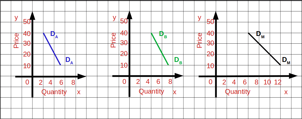
DA and DB are the individual demand curves of individual A and individual B. MD is the market demand curve.
Adding up of Two Linear Demand Curves Given below are the demand equations of two consumers.
$$ {\,d_1(P) \,=\,10\,-\,P}\, ; \,{0\,≤\,P\,≤\,10}$$
$$ {\,= \,0\,;\,P\,>\,0} $$
$$ {\,d_2(P) \,=\,15\,-\,P}\, ; \,{0\,≤\,P\,≤\,15}$$
$$ {\,= \,0\,;\,P\,>\,0} $$
If the price of the commodity is ₹10 or more the first consumer’s demand would be O. Similarly, if the price of the second commodity is ₹15 or more the second consumer’s demand would be O. To find the market demand we have to add these two individual demand equations.
Market demand equation (d(M))
$$ {\,d_1(P) \,+\,d_2(P) \,=\,10\,-\,P\,+ \,15\,-\,P}$$
$$ {d_(m)\, = 25 \,-\,2P\,;\,0\,≤\,P\,≤\,\frac{25}{2}} $$
$$ {0\, = 25 \,;\,P\,>\,\frac{25}{2}} $$


