
Indifference Curve Indifference Curve is defined as the locus of points of combinations of two goods, good 1 and good 2, which gives the consumer the same level of satisfaction. It is the graph showing the bundles that give the consumer the same level of satisfaction. This is shown in below given diagram.
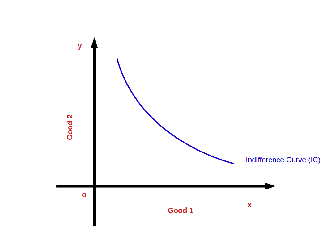
Points on, above and below the indifference curve
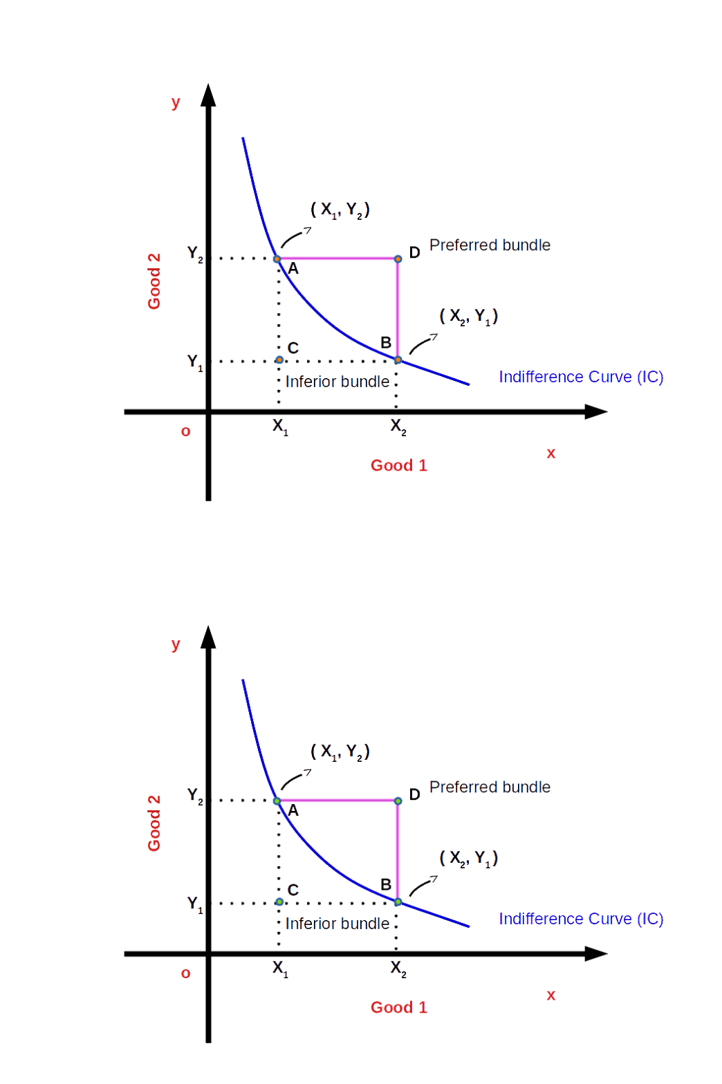 In the above given Diagram, A and B are two points on the indifference curve. The consumption bundles (X1, Y2) and (X2, Y1) give him the same level of satisfaction. The bundles A and B are known as efficient bundles. Any bundle outside the indifference curve, e.g., the bundle at point D is the preferred bundle. But any bundle below the indifference curve is an inferior bundle. For example, C is an inferior bundle.
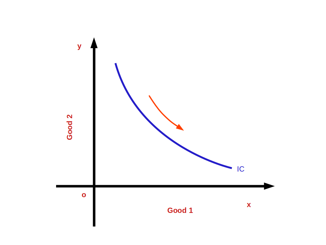
The Rate of Substitution and the Slope of Indifference Curve The slope of indifference curve is equal to the rate of substitution. When the amount of good 1 increases by one unit, the amount of good 2 decreases by same unit. The rate of substitution or Marginal Rate of Substitution (MRS) is the absolute value of the ratio of the good sacrificed and the good obtained. This is the same as the slope of the indifference curve. This is shown in the below Diagram.
Slope of the indifference curve = Rate of Substitution = Marginal Rate of substitution = \(\mathbf{\frac{ΔX_2}{ΔX_1}} \)
As the indifference curve slopes down,
\( \mathbf{{MRS_{x1x2}}\,=\, -\,{\frac{ΔX_2}{ΔX_1}}} \)
Diminishing Marginal Rate of Substitution (DMRS) As the consumer moves along the indifference curve from left to right, the amount of good 1 increases and the amount of good 2 decreases. The marginal rate of substitution between good 1 and good 2 goes on decreasing. This is known as Diminishing Marginal Rate of Substitution (DMRS).
| Table 2.5 | |||
| Bundles | Good 2 (x2) | Good 1 (x1) | MRSx1x2 = \( \bigl( {\frac {Δx_2}{Δx_1}} \bigr) \) |
|---|---|---|---|
| a | 11 | 1 | - |
| b | 7 | 2 | 1:4 |
| c | 4 | 3 | 1:3 |
| d | 2 | 4 | 1:2 |
| e | 1 | 5 | 1:1 |
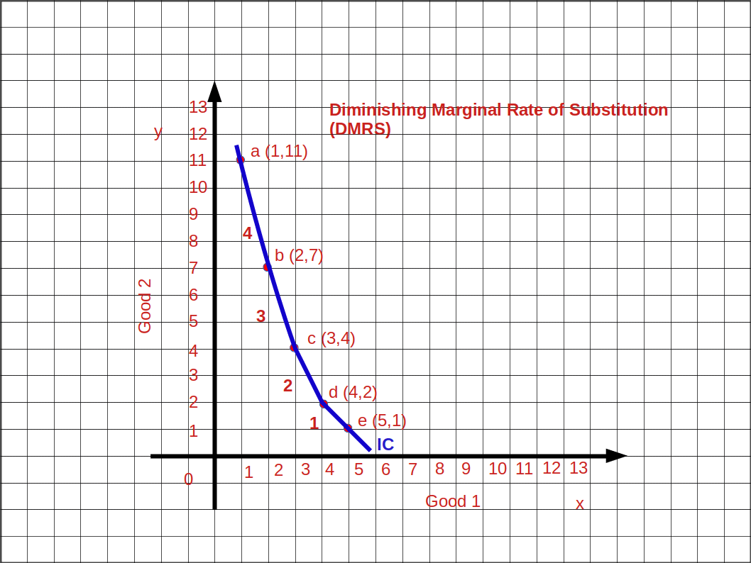
In the Table 2.5 when the consumer moves from bundle a to b, b to c, c to d and d to e, MRS goes on decreasing. MRSx1x2 4, 3, 2, 1. This is shown in the above Graph.
Indifference Map A collection of indifference curves is known as Indifference Map. The below given Diagram shows an indifference map.
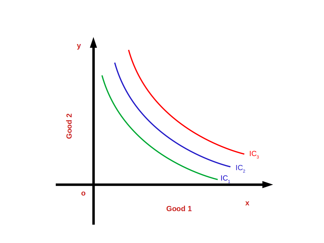
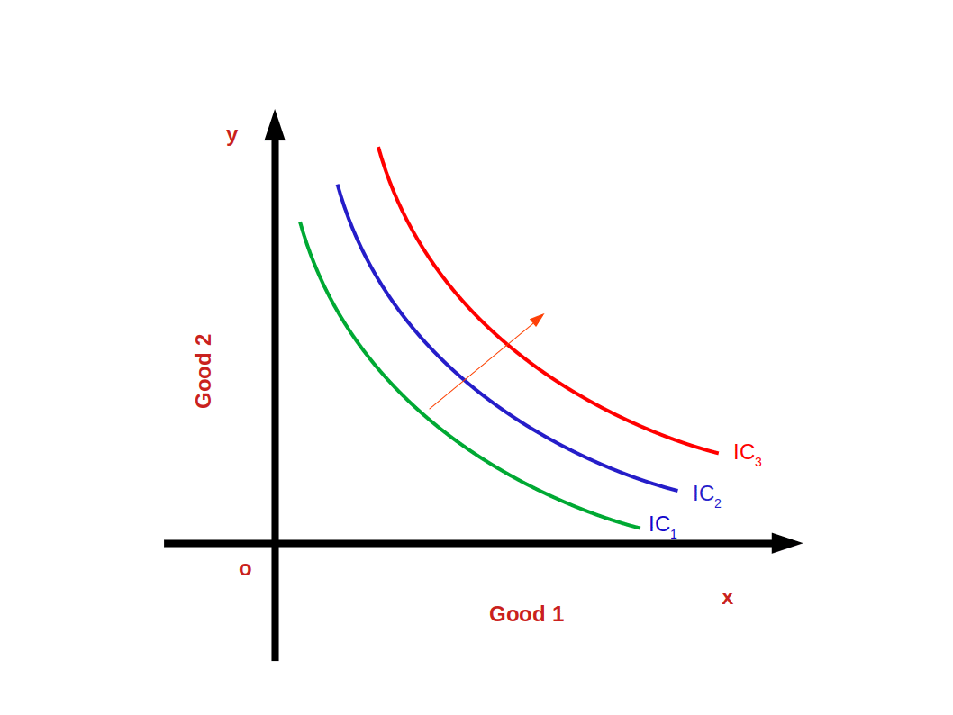
The satisfaction derived from the bundles on the indifference curves IC1, IC2 and IC3 are different. IC2 gives more satisfaction than IC1. IC3 gives much more satisfaction than IC2.
$$ \mathbf{IC_3 > IC_2 > IC_1} $$
Properties (Features) of Indifference Curves
- Indifference curves slope down wards from left to right.
- Indifference curves are convex to the origin. (Because of diminishing marginal rate of substitution).
- Higher indifference curves represent higher levels of satisfaction.
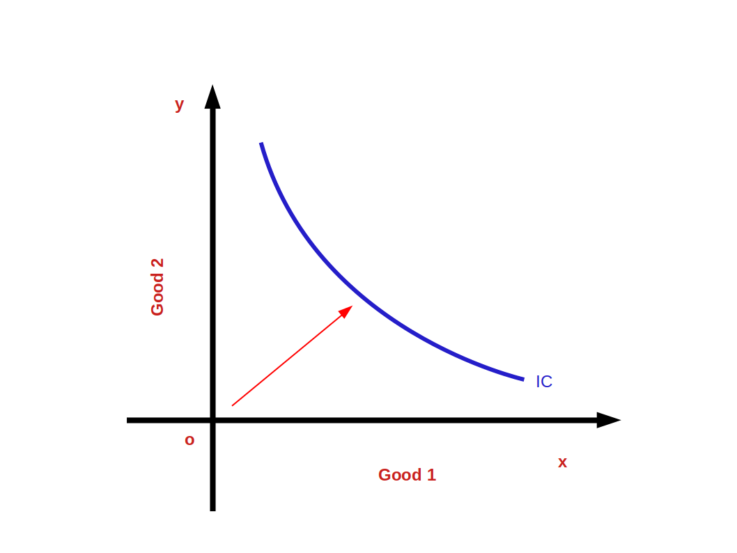
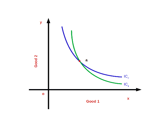
- Indifference curves do not intersect each other. This can be proved with the help of given below diagram. As per the diagram, point a which lies on IC1 and IC2 gives the same level of satisfaction. This is not true. IC2 represents higher level of satisfaction than IC1.
Utility The power of a commodity to satisfy human wants is called utility.
The numbers given to the bundles are called utilities of the bundles. The representation of preferences in terms of utility numbers is called a utility function or a utility representation. The most preferred bundle gets higher utility numbers and the least preferred bundle gets lower utility numbers. Indifferent bundles may have same utility numbers. Table 2.6 gives the utility representation.
| Table 2.6 | |||
| Bundles of two goods | Utility representation | ||
| (2, 2) | 40 units | ||
|---|---|---|---|
| (1, 3), (3, 1), 0, 4), (4, 0) | 35 units | ||
| (1, 2), (2, 1), (0, 3), (3; 0) | 28 units | ||
| (0, 2), (2, 0), (1, 1) | 20 units | ||
| (0, 0), (0, 1), (1, 0) | 10 units | ||
The utility number assigned to the bundle (2, 2) is 40. The utility number assigned to the bundles (1, 3), (3, 0), (0, 4) and (4, 0) is 35. The utility number assigned to the bundles (1, 2), (2, 1), (0, 3) and (3, 0) is 28 and so on. The bundle (2, 2) has the highest utility number because it is the most preferred bundle. On the other hand, the bundles (0, 0) (0, 1) and (1, 0) have lower utility number 10.
Consumer's Equilibrium
(Consumer Optimum) Consumer’s equilibrium can be defined as the position of maximum satisfaction.
According to indifference curve approach, a consumer attains equilibrium at the point where budget line is tangent to indifference curve or MRS equals price ratio or slope of indifference curve (MRS) is equal to slope of budget line, i.e., price ratio \( \bigl( {\frac {- P_1}{P_2}} \bigr) \)
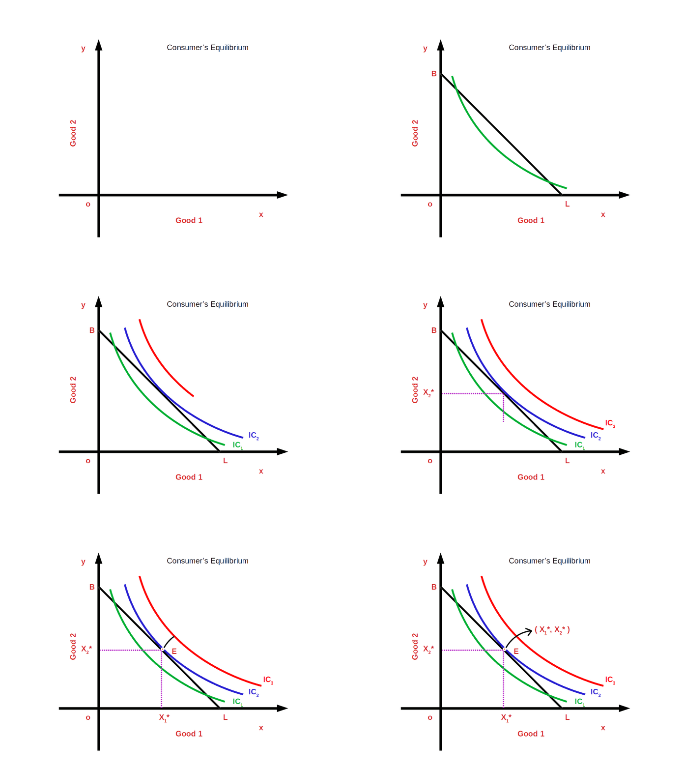
Look at the above given Diagram. BL is the budget line and IC1, IC2, and IC3, are different indifference curves. At point E the slope of the budget line and the slope of IC, become equal \( \bigl( {\frac {Δx_2}{Δx_1}}\, = \, MRS_{x1x2}\, = \, {\frac {- P_1}{P_2}} \bigr) \). At point E, the consumer is at equilibrium. As he chooses the bundle (x1*, x2*) he gets maximum satisfaction.
The consumption bundles on IC1 give less satisfaction than the bundles on the indifference curve IC2. The bundles on IC3 give more satisfaction than the bundles on indifference curve IC2. The consumer cannot get the bundles on IC3 because all the bundles on IC3 are beyond his budget line. Therefore, the bundle (x1*, x2*) gives him the maximum Satisfaction.


