
Introduction: The theory of consumer behaviour analyses how a consumer maximises his satisfaction from his consumption expenditure.
 Consumers buy or demand goods and services to satisfy their wants. They. can satisfy their wants by consuming goods. Goods are bought by consumers to reach the highest level of satisfaction, i.e., consumer’s equilibrium. Consumers have to decide what quantity of a good they should buy at a given price and at a given point of time. In other words, we have to study consumer behaviour. To understand consumer behaviour, first we have to understand the concept utility. Utility is the want Satisfying power of a commodity or service. There are three important theories that explain the measurement of utility and the process that leads to consumer’s equilibrium. They are:
- Cardinal utility approach of Alfred Marshall
- Ordinal utility approach of J. R. Hicks
- Revealed preference Hypothesis of Paul A. Samuelson


Here we discusses how a consumer achieves consumer’s equilibrium according to the ordinal utility approach. Ordinal utility approach is also known as Indifference curve approach.
Consumption Bundle
A consumer cannot buy every thing he/she wants. Since wants are unlimited, he/she has to make a choice. Normally consumers buy many goods. But for ease of analysis let us assume that there are only two goods. They are good 1 and good 2. Any combination of the amount of two goods is called a consumption bundle. Let x1 be the amount of good 1 and x2 amount of good 2. (x1, x2) can be called consumption bundle.
 Bundle (4, 6) contains 4 units of good 1 and 6 units-ef good 2. Similarly, bundle (10, 15) contains 10 units of good 1 and 15 units of good 2.
Consumer’s Budget
Consumer’s budget is the income or amount of money available for spending on either goods as he wishes. The consumer can spend his entire income either on good 1 or on good 2 or combination of both. ‘Consumer’s budget is the money income of the consumer which he can use to buy goods and services.
To buy sugar and tea Sindhu has ₹100 and Sethu has ₹75. Let us Find Sindhu’s and Sethu’s budget. Here we can say that Sindhu's budget is ₹100 and Sethu's budget is ₹75.
Budget Set
A set of consumption bundles is known as budget set. In other words, it is defined as the collection of all the bundles that the consumer can buy with his income at the prevailing market prices.
Consumer’s behaviour is constrained by his budget. His expenditure should be less than or equal to his budget. Budget constraint can be defined algebraically as P1x1 + P2x2 ≤ M, where, P1 = Price per unit of good 1, P2 = Price per unit of good 2, x1 = Number of units of good 1, x2 = Number of units of good 2 and M = Money income available to the consumer. The inequality P1x1 + P2x2 ≤ M is called Consumer’s Budget Constraint.
Budget Constraint = \( \mathbf{{{P_1 X_1 + P_2 X_2 ≤ M} }} \)
 Let us explain this using an example. Suppose a consumer has ₹20 to spend on two goods. The price per unit of good 1 and good 2 is ₹5. Then the budget set equation is 5x1 + 5x2 ≤ 20. As per this budget set of consumer, the following are the available bundles of good 1 and good 2 which cost less than or equal to ₹20.
{(0, 0), (0, 1), (0, 2), (0, 3), (0, 4), (1, 0), (1, 1), (1, 2), (1, 3), (2, 0), (2, 1), (2, 2), (3, 0), (3, 1), (4, 0)}
These bundles can be plotted in a graph.
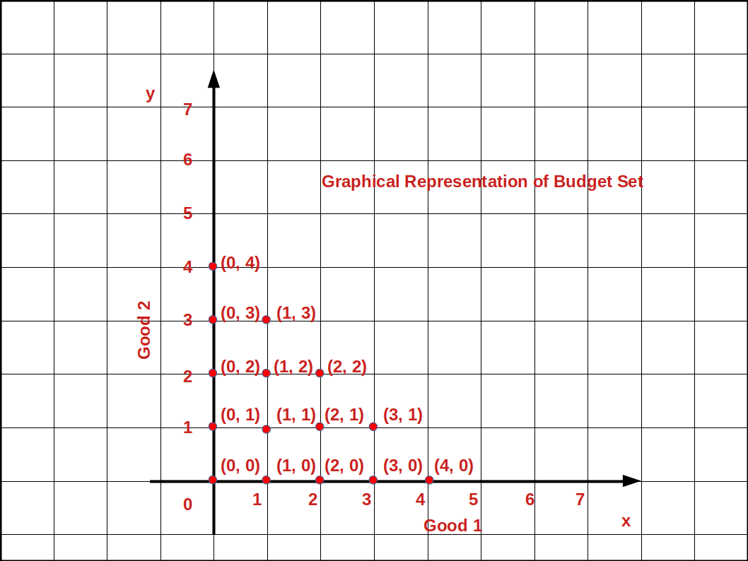 In the above given graph, bundles (0, 4) (1, 3) (2, 2) (3, 1) and (4, 0) are cost exactly equal to ₹20. All other bundles cost less than ₹20.

Budget Line
Budget line is defined as the locus of points of combinations of good 1 and good 2 which cost exactly equal to income. In other words, budget line is the line which consists of all the bundles or combinations that cost exactly equal to the consumer’s income. Algebraically,
Budget Line = \( \mathbf{{{P_1 X_1 + P_2 X_2 = M} }} \)
If the consumer spends his entire income on good 1, he can buy \( \mathbf {{{{\frac{M}{P_1}} }}} \) units of good 1. On the contrary, if he spends the entire income on good 2 he can buy \( \mathbf {{{{\frac{M}{P_2}} }}} \) units of good 2.
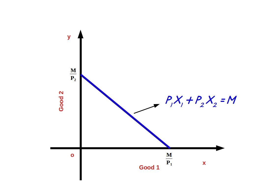
If we represent good 1 on x-axis and good 2 on y-axis, \( \mathbf {{{{\frac{M}{P_1}} }}} \) (the point where budget line touches x-axis) becomes the horizontal intercept and \( \mathbf {{{{\frac{M}{P_2}} }}} \) (the point where budget line touches y-axis) becomes vertical intercept as shown in above diagram.
How to find Horizontal intercept and Vertical intercept ?
Consider the budget line P1x1 + P2x2 = M
If x2 = 0 ie., the consumer does not buy good 2, the quantity of x1 would be:
P1x1 + P2 × 0 = M
P1x1 = M
\( \mathbf {x_1 \, = \, {{{{\frac{M}{P_1}}} }}} \) or \( \mathbf{( {{{{\frac{M}{P_1}}, 0 ) } }}} \) is the horizontal intercept. This is the point where budget line touches x-axis.
If x1 = 0 i.e., the consumer does not buy good 1, the quantity of x2 is
P1 × 0 + P2x2 = M
P2x2 = M
\( \mathbf {x_2 \, = \, {{{{\frac{M}{P_2}}} }}} \) or \( \mathbf{(0, {{{{\frac{M}{P_2}} ) } }}} \) This is the vertical intercept where budget line touches y-axis.
Let us practice an example. In the budget line equation
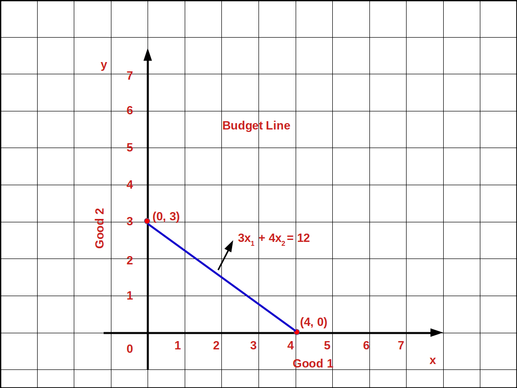
3x1 + 4x2 = 12, if X2 = 0
3x1 + 4 × 0 = 12,
3x1 = 12
x1 = \( \mathbf {{{{\frac{12}{3}} }}} = 4 \) is the horizontal intercept, i.e., (4, 0).
if x1 = 0, 3 × 0 + 4x2 = 12
4x2 = 12
x2 = \( \mathbf {{{{\frac{12}{4}} }}} = 3 \) is the vertical intercept., i.e., (0, 3)
The budget line 3x1 + 4x2 = 12 is shown in the below graph.
There is an another method to find budget line equation.
Solve the equation P1x1 + P2x2 = M for x2
i.e., P2x2 = M - P1x1
x2 = \( {{{{\frac{M - P_1x_1}{P_2}} }}} \)
x2 = \( {{{{{\frac{M}{P_2}}} - {\frac{P_1}{P_2}} }}} x_1\)
\( {\frac{M}{P_2}} \) is the vertical intercept, \( - {\frac {P_1}{P_2}} \) is the slope of the budget line.
Let us practice an example. Consider the budget line equation 5x1 + 5x2 = 20
When we solve for x2
5x1 + 5x2 = 20
5x1 + 5x2 = 20 - 5x1
x2 = \( {{{{\frac{20 - 5x_1}{5}} }}} \)
= \( {{{{{\frac{20}{5}}} - {\frac{5x_1}{5}} }}} \)
x2 = 4 - x1
In this form of the budget line the vertical intercept is 4 and the slope is -1.
The Table 2.1 shows the different bundles that can be bought with = 20 using the equation x2 = 4 - x1.
| Table 2.1 | ||
| x1 | x2 = 4 - x1 | Bundles |
|---|---|---|
| 0 | 4 - 0 = 4 | (0, 4) |
| 1 | 4 - 1 = 3 | (1, 3) |
| 2 | 4 - 2 = 2 | (2, 2) |
| 3 | 4 - 3 = 1 | (3, 1) |
| 4 | 4 - 4 = 0 | (4, 0) |
In the below Graph we have different bundles of (0, 4) (1, 3) (2, 2) (3, 1) (4, 0).

When these bundles are joined with a line, it is called budget line. The cost of all these bundles is exactly equal to the consumer’s income of ₹20.
Points on, above and below the Budget line
In any of the bundles or points below the budget line the consumer does not spend all his income. He has some money unused. Using this amount he can buy more units of good 1 or good 2 or both.

In the above Diagram points A, B, C are on the budget line. Point D is below the budget line and point E is outside the budget line. At point A he buys 1 unit of good 1 and 3 units of good 2 (1, 3). At point B he buys 2 units of good 1 and 2 unit of good 2 (2, 2) and at point C he can buy 3 units of good 1 and 1 unit of good 2 (3, 1). The bundles A B and C are known as efficient bundles. But at point D he buys 1 unit of good 1 and 1 unit of good 2 (1, 1). Then his expenditure at point D will be less than his income. This bundle is called inferior bundle. But point E is outside the budget line. To buy goods at this point the consumer’s income will not be enough. But this bundle would be superior to the bundle on the budget line. This bundle is known as superior bundle or preferred bundle.

- Any point on budget line indicates combinations of good 1 and good 2 a consumer can purchase which cost an amount exactly equal to his income. This bundle is known as efficient bundle.
- Any point below. budget line indicate combination of good 1 and good 2 a consumer can purchase which costs less than his income. This bundle is known as inferior bundle.
- Any point above budget line indicates combination of good 1 and good 2 a consumer is unable to purchase with his limited income. This bundle is known as ‘Superior or preferred bundle.
Slope of the Budget Line and the Price Ratio
The amount of good 2 sacrificed to buy one extra unit of good 1 is called slope of the budget line. It is calculated by dividing the change (Δx2) in good 2 by change in good 1 (Δx1). The slope of the budget line will always be a negative number because it slopes downward from left top to right bottom.
Every point on the budget line shows the bundles in which the consumer’s income is completely spent. Therefore, in order to get one additional unit of good 1, the consumer has to give up some unit of good 2. To get one extra unit of good 1 how many units of good 2 should the consumer sacrifice? It depends on the prices of both goods. If the price of good 1 is P1 the consumer has to educe the expenses for good 2 by P1. The consumer can buy \( {\frac {P_1}{P_2}} \) units of good 2 with P1 i.e., the consumer can substitute good 1 for good 2 at the rate of \( {\frac {P_1}{P_2}} \). Then the slope of the budget line shows the price ratio of two goods. Therefore, we can define the slope of the budget line as
\( \mathbf {{{\frac {Δx_2}{Δx_1}}} = {- {\frac {P_1}{P_2}}}} \)
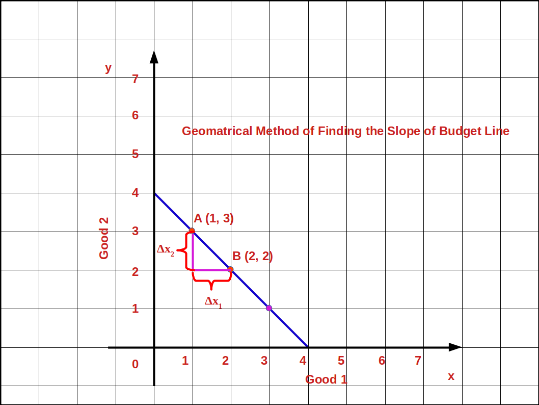
In the above given graph, when the consumer moves from bundle A to bundle B the decrease in good 2 is (Δx2) 1 unit. The increase in good 1 is (Δx1) 1 unit. Therefore, the slope of the budget line is \( {{{\frac {Δx_2}{Δx_1}}} = {{\frac {2 - 3}{2 - 1}}} = {{\frac {- 1}{1}}}} = -1\)
Changes in Budget Set
The consumption bundles available to a consumer depends on: (I) changes in the income of the consumer and (II) changes in the prices of goods. Therefore, any change in the prices of goods or income of the consumer may affect the budget set and budget line.
(I) Changes in the Income of the consumer
There are two types of changes in the income of the consumer. They are
- Increase in income and
- Decrease in income
a. Increase in income
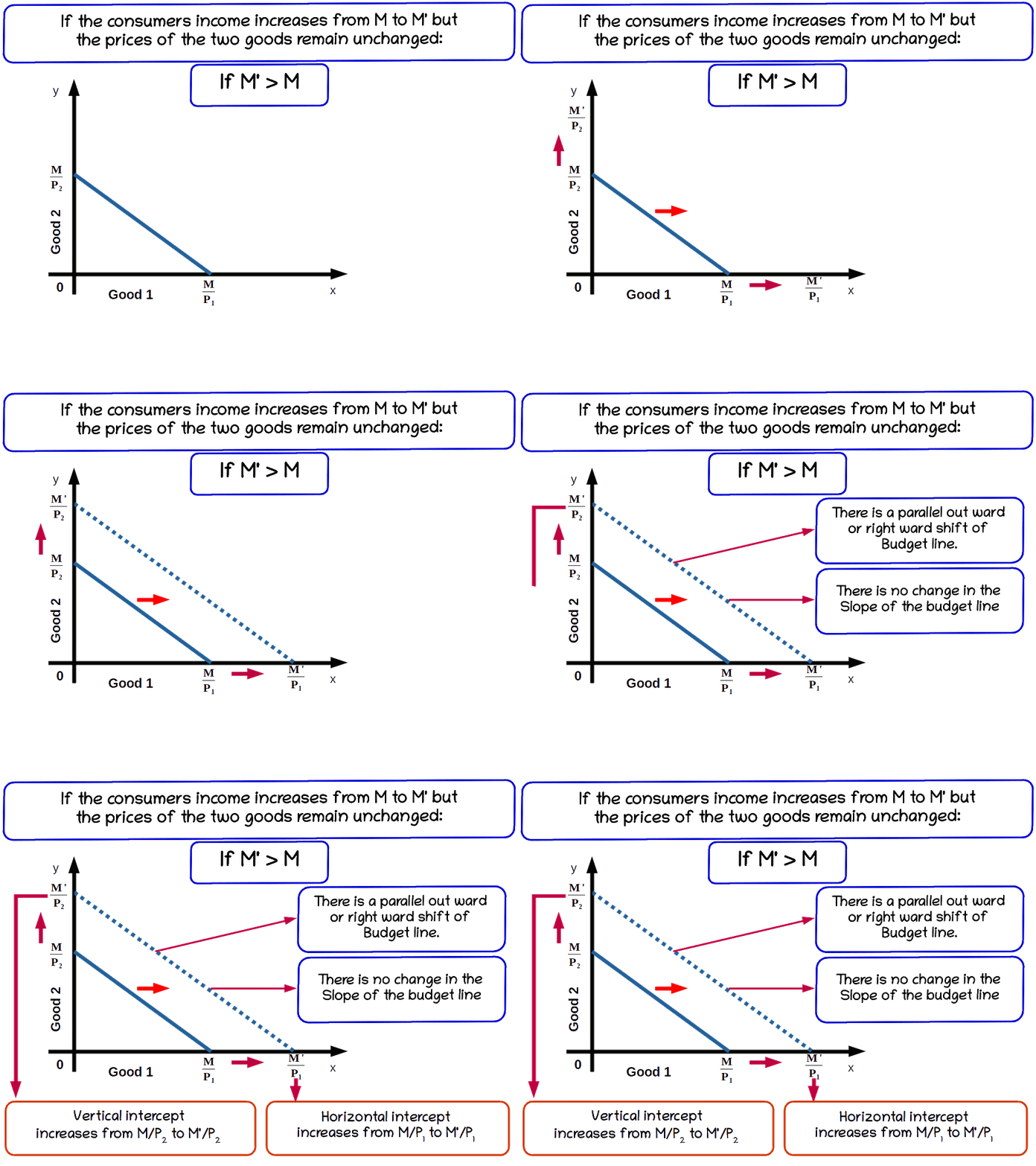
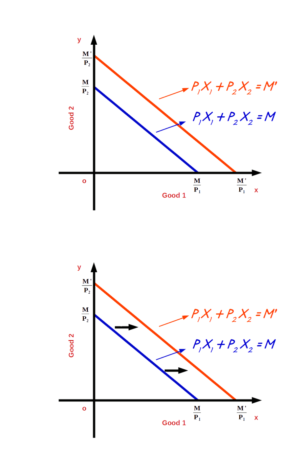
When the income of the consumer increases, the consumer is able to buy more of two goods and the budget line shifts parallel outward. If his income increases from M to M’ the new budget line equation would be P1x1 + P2x2 = M' and the vertical intercept of this budget line would be \( {\frac {M'}{P_2}} \) and horizontal intercept would be \( {\frac {M'}{P_1}} \). Budget lines with incomes M and M' are given in below diagram.
Let us practice an example. Suppose the consumer’s income increases from ₹20 to ₹30 and the prices of good 1 and good 2 remain the same as ₹5. Then the new budget line equation would be 5x1 + 5x2 = 20. The vertical intercept and the horizontal intercept would be 6. When income increased from ₹20 to ₹30 vertical and horizontal intercepts shifted from 4 to 6, refer the below given graph.
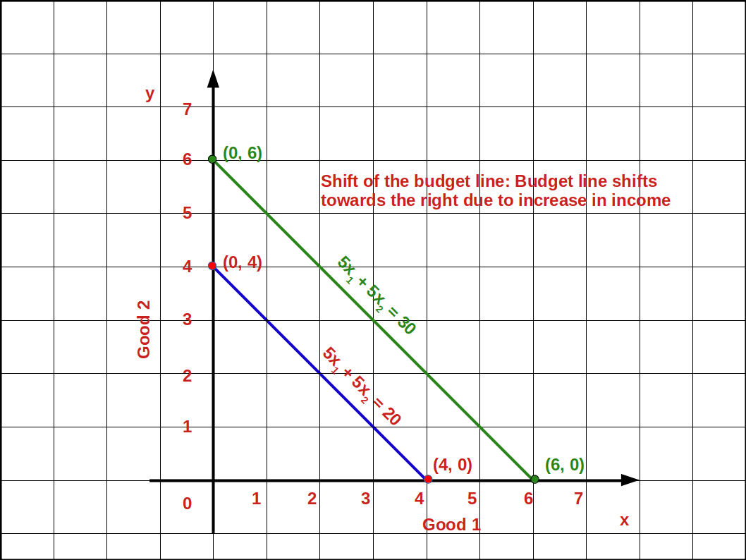
The budget line shifts from 51 +52 =20 to 51 +52 =30. Now the consumer can buy extra units of both goods. The slope of budget line \( {\frac {-P_1}{P_2}} \) remains -1.
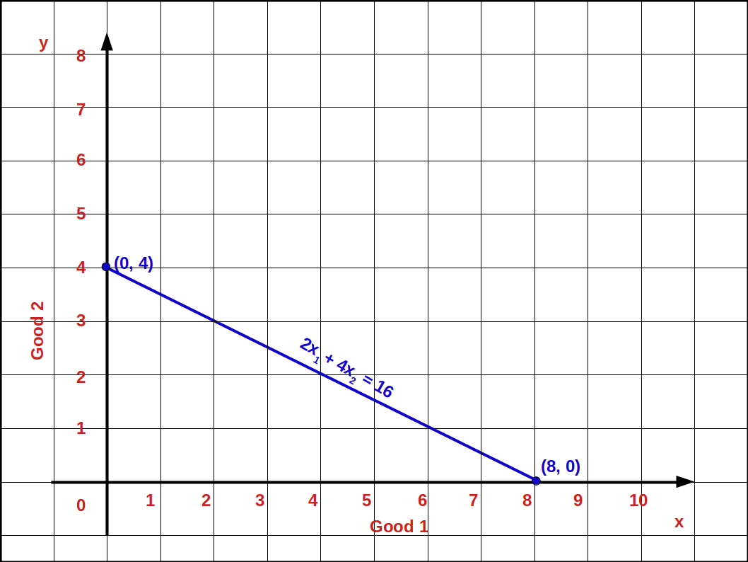
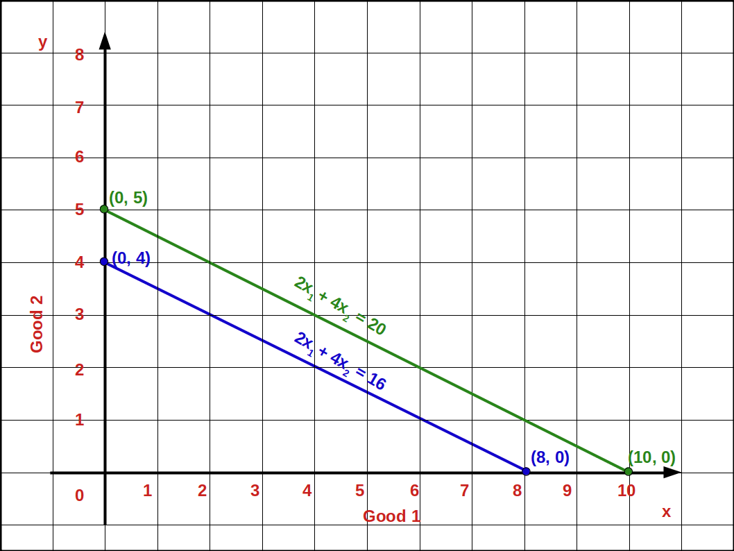
Let us practice an example. If P1 = 2, P2 = 4, M = 16.
- Write down the budget line equation.
- Find vertical intercept.
- Find horizontal intercept.
- What is the slope of the budget line ?
- Draw the budget line.
- M = 16 changes to M’ = 20. What happens to budget line? Draw the budget line.
- What is the slope of the new budget line ?
- 2x1 + 4x2 = 16
- Vertical intercept \( {{\frac {M}{P_2}} = {\frac {16}{4}}} =\,4 \) (0, 4)
- Horizontal intercept \( {{\frac {M}{P_1}} = {\frac {16}{2}}} =\,8 \) (8, 0)
- Slope \( {\frac {Δx_2}{Δx_1}} \)
= \( {\frac {-P_1}{P_2}} \)
= \( {\frac {-2}{4}} \)
= \( {\frac {-1}{2}} =\,-\,0.5 \)
-
- Vertical intercept \( {{\frac {M'}{P_2}} = {\frac {20}{4}}} =\,5 \) (0, 5)
- Horizontal intercept \( {{\frac {M'}{P_1}} = {\frac {20}{2}}} =\,10 \) (10, 0)
- \( -{\frac {P_1}{P_2}} \)
\( -{\frac{2}{4}} \)
\( {-\frac {1}{2}}=\,-\,0.5 \)
b. Decrease in income
When the consumer’s income decreases, he is not able to buy goods with the same amount. So the budget line shifts parallel leftward. When income decreases from M to M'1 (M'1 < M) the budget line shifts to the left. It is shown in the below Diagram.

| Table 2.2 Changes in Budget Line | ||
| Increase in Income | Decrease in Income | |
| M < M' | M > M'1 | |
|---|---|---|
| Budget line equation P1x1 + P2x2 = M' | Budget line equation P1x1 + P2x2 = M'1 | |
| Vertical intercept moves up from \( \mathbf{\frac {M}{P_2}} \) to \( \mathbf{\frac {M'}{P_2}} \) | Vertical intercept moves down from \( \mathbf{\frac {M}{P_2}} \) to \( \mathbf{\frac {M'_1}{P_2}} \) | |
| Horizontal intercept moves up from \( \mathbf{\frac {M}{P_1}} \) to \( \mathbf{\frac {M'}{P_1}} \) | Horizontal intercept moves up from \( \mathbf{\frac {M}{P_1}} \) to \( \mathbf{\frac {M'_1}{P_1}} \) | |
| Consumer is able to purchase more quantities of both goods | Consumer is not able to purchase more quantities of both goods | |
| Budget line shift rightward | Budget line shift leftward | |
| Slope does not change | Slope does not change | |
Let us try to answer the below given problem.
The income of budget line 1 is ₹12 and that of the second one is ₹20. The slope of the first budget line equals the slope of the second budget line.
That is, \( -\,{\frac {P_1}{P_2}} \) = \( -\,{\frac {3}{4}} \) slope.
This is because there is no change in the prices of both the goods.
(II) Changes in Price
If price of goods changes without any change in consumer’s income, there will be changes in vertical - horizontal intercepts and slopes. There are two types of changes in the price of good 1. They are,
- Increase in price of good 1
- Decrease in price of good 1
- Increase in price of good 2
- Decrease in price of good 2
a. Increase in price of good 1
If the price of good 1 increases from P1 to P’1 and the price of good 2 and income of the consumer (M) remains unchanged, horizontal intercept of the budget line pivots inwards around the y-axis and the slope increases. Consumer is not able to buy good 1 with the same amount.
When price of good 1 increases from P1 to P'1, P'1x1 + P2x2 = M, is the equation of the budget line. Here, \( {\frac {M}{P_2}} \) is the vertical intercept and \( {\frac {M}{P_1}} \) is the horizontal intercept \( - {\frac {P_1}{P_2}} \) becomes the slope of the budget line. This is shown in the below given Diagram. Here we can see that due to an increase in price of good 1 horizontal intercept \( {\frac {M}{P_1}} \) moves inward to \( {\frac {M}{P'_1}} \). Moreover, there is no change in vertical intercept. It remains the same as \( {\frac {M}{P_2}} \).

Let us practice an example.
Price of good 1 increases from ₹5 to ₹10. Price of good 2 is ₹5 and the consumer’s income is ₹20. The new budget line would be 10x1 + 5x1 = 20.
Vertical intercept = 4 = \( \Bigl({\frac {M}{P_2}} = {\frac {20}{5}} = 4 \Bigr)\).
Horizontal intercept= 2 = \( \Bigl({\frac {M}{P'_1}} = {\frac {20}{10}} = 2 \Bigr)\).
The slope of the budget line is -2 because in order to get one unit of good 1, 2 units of good 2 have to be sacrificed. 5x1 + 5x2 = 20 is the old budget line and 10x1 + 5x1 = 20 is the new budget line as is shown in the below given graph. Here, we can see that the horizontal intercept of the new budget line has moved towards vertical axis.

b. Decrease in price of good 1
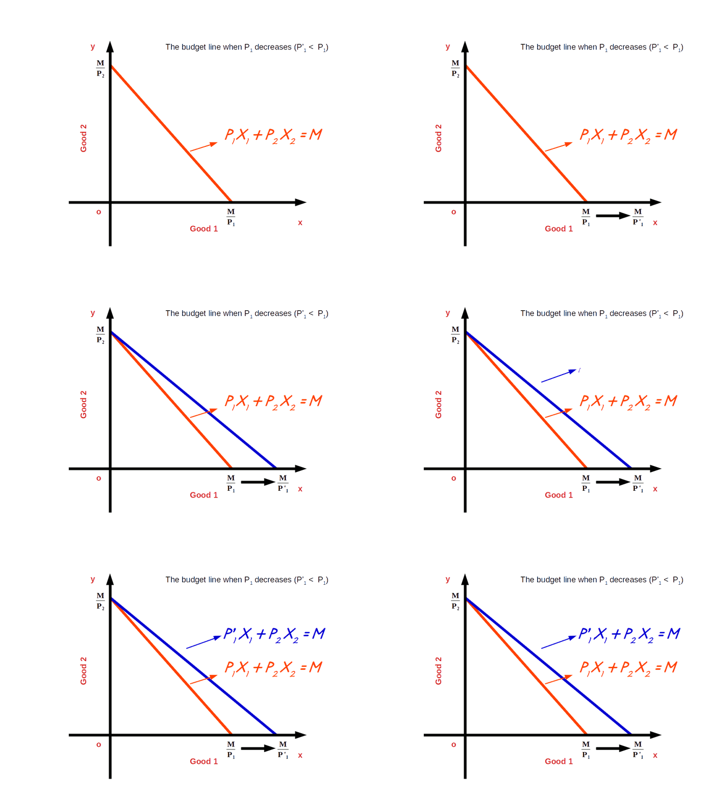
If the price of good 1 decreases from P1 to P’1 and the price of good 2 and income of the consumer (M) remain unchanged, horizontal intercept of the budget line pivots-outwards around the y-axis and the slope decreases. Consumer is able to buy more of good 1 and the budget line becomes less steep. This situation is shown in the below digram.
Let us practice an example.
In the budget line equation 5x1 + 5x2 = 20 if the price of good 1 decreases from ₹5 to ₹4 the vertical intercept of the new budget line, 4x1 + 5x2 = 20 will be 4 \( \Bigl({\frac {M}{P_2}} = {\frac {20}{5}} = 4 \Bigr)\).
The horizontal intercept will increase to 5 from 4 \( \Bigl({\frac {M}{P'_1}} = {\frac {20}{4}} = 5 \Bigr)\).
And the slope of the budget line changes from 1 to 0.8 \( \Bigl(-{\frac {P'_1}{P_2}} = -{\frac {4}{5}} = -0.8 \Bigr)\). Look at the budget line drawn in the below graph.

c. Increase in price of good 2
If the price of good 2 increases from P2 to P’2 and the price of good 1 and income of the consumer (M) remains unchanged, vertical intercept of the budget line pivots inwards around the x-axis and the slope decreases. Consumer is not able to buy good 2 with the same amount.
When price of good 2 increases from P2 to P'2, P1x1 + P'2x2 = M, is the equation of the budget line. Here, \( {\frac {M}{P_2}} \) is the vertical intercept and \( {\frac {M}{P_1}} \) is the horizontal intercept \( - {\frac {P_1}{P_2}} \) becomes the slope of the budget line. This is shown in the below given Diagram. Here we can see that due to an increase in price of good 2 horizontal intercept \( {\frac {M}{P_2}} \) moves inward to \( {\frac {M}{P'_2}} \). Moreover, there is no change in vertical intercept. It remains the same as \( {\frac {M}{P_1}} \).

d. Decrease in price of good 2
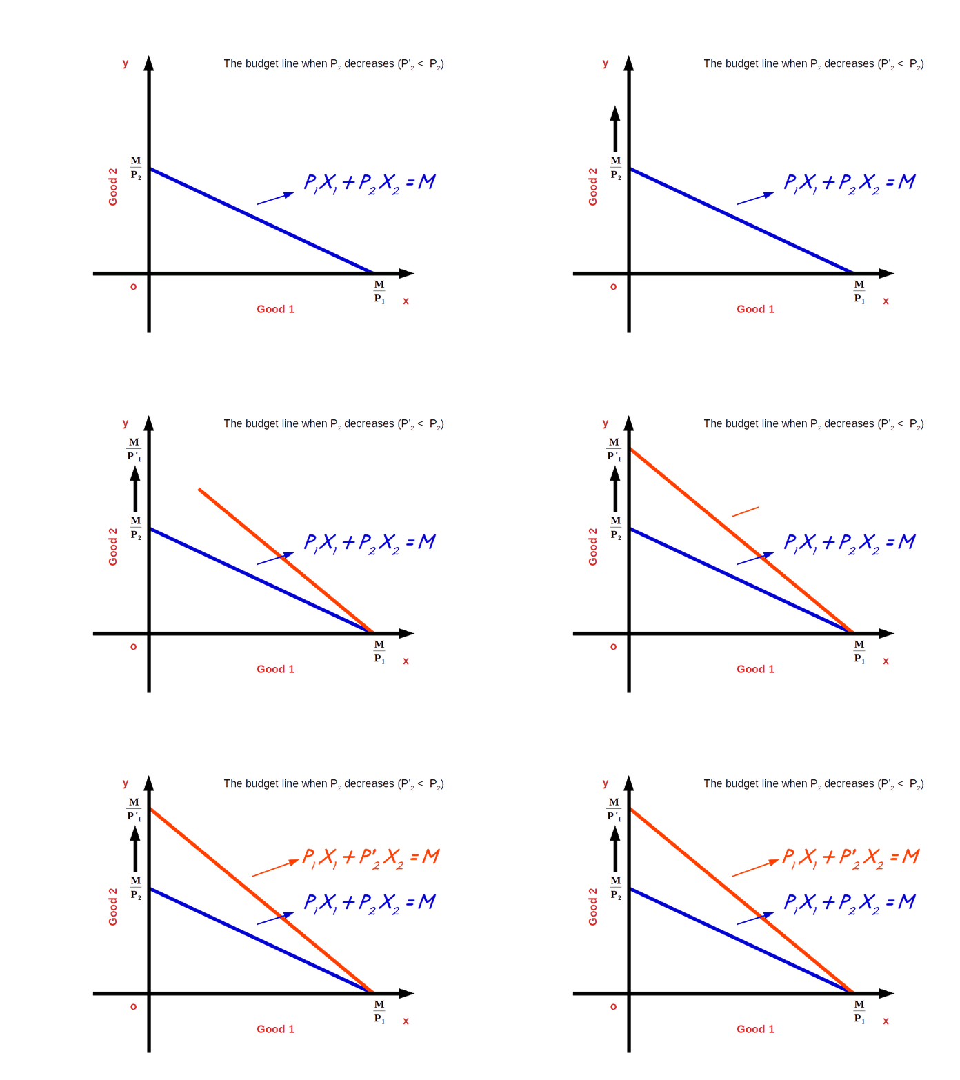
If the price of good 2 decreases from P2 to P’2 and the price of good 1 and income of the consumer (M) remain unchanged, vertical intercept of the budget line pivots-outwards around the x-axis and the slope increases. Consumer is able to buy more of good 2 and the budget line becomes more steep. This situation is shown in the below digram.
Preferences of the Consumer
The consumer chooses his consumption bundles from the budget set depending on his taste and preferences over the bundles. He compares the consumption bundles. And between any two consumption bundles, he prefers one bundle to the other or he is indifferent. The consumer ranks the bundles in the order of his preferences from the best to the least.
Consumption bundles as per budget set 5x1 + 5x2 ≤ 20 are ranked below in the order of preference.
| Table 2.3 | |
| Bundles | Ranking |
| (2, 2) | I |
|---|---|
| (1, 3), (3, 1) | II |
| (1, 2), (2, 1) | III |
| (1, 1) | IV |
| (0, 1), (0, 2), (0, 3), (0, 4), (1, 0), (2, 0), (3, 0), (4, 0) | V |
In the above Table most preferred bundle is (2, 2). Bundles (1, 3), (3, 1) are similar to the consumer. These bundles give the same level of satisfaction. Ranking or preferences will change according to personal preferences.
Monotonic Preference
Consumer’s preferences are said to be monotonic preferences, if between any two bundles, the consumer prefers the bundle which has more of at least one of the goods and no less of the other goods as compared to the other bundles. (x1, x2) and (y1, y2), are two bundles; if (x1, x2) has more of at least one of the goods and no less of the other goods as compared to (y1, y2), the consumer prefers (x1, x2) to (y1, y2). Simply monotonic preference means, the consumer prefers more amount of bundle than less amount of bundle and is called monotonic preference. In other words consumer prefers the superior bundle to the inferior bundle, when his preference is monotonic.
In Table 2.3, the consumer prefers (2, 2) to (2, 1). This is because in the bundle (2, 2) we have 1 unit more of good 2 as compared to the bundle (2, 1). If the consumer chooses the bundle (2, 1), his preference is not monotonic.
Substitution between Goods
Substitution between goods means the amount of good 2 that the consumer is willing to give up to get one unit of good 1. The rate at which one good is substituted for another is called rate of substitution.
It measures the consumers willingness to pay for good 1 in terms of good 2. The rate of substitution between good 2 and good 1 is given by the absolute value of Δx2 ÷ Δx1 where Δx2 represents change in good 2 and Δx1 represents change in good 1.
We can explain it with an example. Consider the bundles (2, 2) and (1, 3). Δx2 = (3 - 2) = 1 and Δx1 = (2 - 1) = 1. Therefore \( \vert{\frac {Δx_2}{Δx_1}} \vert\) = \( {\frac {1}{1}}\,=\,1\). Thus the rate of substitution between good 2 and good 1 is 1.
Diminishing Rate of Substitution
Let us assume that a consumer consumes two goods, good 1 and good 2. To obtain more units of good 1, he has to sacrifice some units of good 2. As the consumer consumes more and more units of good 1, the amount of good 2 sacrificed diminishes. This is known as Diminishing Rate of Substitution. The consumer's preference of this kind is called convex preferences.
| Table 2.4 | |||||
| Good 1 | Good 2 | Δx1 | Δx2 | Rate of Substitution. \( \bigl( {\frac {Δx_2}{Δx_1}} \bigr) \) | |
|---|---|---|---|---|---|
| 10 | 20 | - | - | - | |
| 11 | 15 | 1 | 5 | 5 | |
| 12 | 11 | 1 | 4 | 4 | |
| 13 | 8 | 1 | 3 | 3 | |
| 14 | 6 | 1 | 2 | 2 | |
| 15 | 5 | 1 | 1 | 1 | |
Look at the above table. All are indifferent bundles. All these bundles give same level of satisfaction. As the consumer substitutes more and more units of good 1 for good 2 the absolute value of rate of substitution declines from 5 to 1.


