Plus Two Economics-Chapter 6
Chapter 6:-


Introduction Price and output determination in non-competitive markets like monopoly, monopolistic competition and oligopoly are discussed here.
Simple Monopoly in the Commodity Market The word ‘Monopoly’ has been derived from the Greek words ‘mono’ which means single and ‘poly’ which means seller. Therefore monopoly means single seller. Monopoly is a market situation in which a single seller or firm controls the entire supply of a product which has no close substitutes. Main features of monopoly are given below:
- Single seller for a product.
- Absence of substitute products.
- Entry of new firms in the market is denied.
- The monopolist has complete control over supply of the product.
- Firm and industry are the same because there is only one firm in the monopoly market.
- The firm is the price-maker.
Market Demand Curve of Monopoly In a monopoly market the firm and the industry are the same. So the firm demand curve and market demand curve would be the same. Demand curve of a monopoly firm will slope negatively as shown in the Diagram.
 The average revenue curve of a monopoly firm is the same as its demand curve, It slopes downwards from left to right. This means, the monopolist firm can sell less quantity at high price and more quantity at lower price. If the monopolist fixes price P0 in the above Diagram, he can sell q0 quantity of output, If the price falls to P1 quantity rises to q1.
Suppose q = 10 – P is the demand function of a monopoly where q is the quantity and P is the price. This equation can be written in terms of P.
q = 10 – P
∴ P = 10 – q
We get P = 10 – q. Now give values to q from 0 to 7. Then price decreases from 10 to 3 as seen in Table 6.1.
As there is only one producer in the monopoly market, supply is completely controlled by that firm. So the monopolist can influence the price. But the monopolist cannot control the price and the quantity of supply simultaneously. If the monopolist determines the quantity of sale, the market will determine the price. Similarly, if the monopolist determines the price, the market will determine the quantity of sale.
The quantities of goods supplied at various prices represent market demand curve in the monopoly market. Therefore, the monopolist’s supply curve represents the market demand curve. In a monopoly market the monopolist can control price. So the firm is called the price-maker, because it can sell less by increasing price or sell more by decreasing price.
The average revenue curve of a monopoly firm is the same as its demand curve, It slopes downwards from left to right. This means, the monopolist firm can sell less quantity at high price and more quantity at lower price. If the monopolist fixes price P0 in the above Diagram, he can sell q0 quantity of output, If the price falls to P1 quantity rises to q1.
Suppose q = 10 – P is the demand function of a monopoly where q is the quantity and P is the price. This equation can be written in terms of P.
q = 10 – P
∴ P = 10 – q
We get P = 10 – q. Now give values to q from 0 to 7. Then price decreases from 10 to 3 as seen in Table 6.1.
As there is only one producer in the monopoly market, supply is completely controlled by that firm. So the monopolist can influence the price. But the monopolist cannot control the price and the quantity of supply simultaneously. If the monopolist determines the quantity of sale, the market will determine the price. Similarly, if the monopolist determines the price, the market will determine the quantity of sale.
The quantities of goods supplied at various prices represent market demand curve in the monopoly market. Therefore, the monopolist’s supply curve represents the market demand curve. In a monopoly market the monopolist can control price. So the firm is called the price-maker, because it can sell less by increasing price or sell more by decreasing price.
TR, AR and MR under Monopoly
Total Revenue – TR. Total revenue is the total amount of revenue earned by a firm by selling output in the market. TR is calculated by multiplying the quantity of output by price (TR = p × q). TR of a monopoly firm is not a straight line. It depends on the nature of demand function. The shape of TR curve is an inverted Parabola as shown in below Diagram.
Average Revenue — AR Average revenue is revenue per unit of sale. AR is calculated by dividing TR by quantity of output sold.
\( \mathbf{AR\,=\,\frac{TR}{Q}\,=\,\frac{P×q}{q}\,=\,P}\)
In monopoly market AR is equal to p. So AR curve and market demand curve would be the same. In Table 6.1 it can be seen that AR and pare equal.
| Table 6.1 | ||||
|---|---|---|---|---|
| q | P = 10 – q | TR = P × q | AR = \(\mathbf{\frac{TR}{q}}\) | MR = \(\mathbf{\frac{ΔTR}{Δq}}\) |
| 0 | 10 | 0 | – | – |
| 1 | 9 | 9 | 9 | 9 |
| 2 | 8 | 16 | 8 | 7 |
| 3 | 7 | 21 | 7 | 5 |
| 4 | 6 | 24 | 6 | 3 |
| 5 | 5 | 25 | 5 | 1 |
| 6 | 4 | 24 | 4 | -1 |
| 7 | 3 | 21 | 3 | -3 |
Derivation of AR from TR curve We can discuss the method of finding AR from TR with the help of below given Diagram. In this diagram quantity is marked along the x-axis and TR is marked on the y-axis. TR is the total revenue curve. Suppose we want to find AR when quantity is ‘b’. Draw a perpendicular .from point ‘b’ to TR curve. It cuts TR at point ‘a’. Draw a line from the origin to a. AR will be the slope of Oa.
 Therefore,
Slope of the line Oa = \(\,\frac{ab}{Ob}\) = AR
Therefore,
Slope of the line Oa = \(\,\frac{ab}{Ob}\) = AR
Marginal Revenue (MR) Marginal Revenue is the addition to the TR, when an extra unit is sold. It is the rate of change of TR. Algebraically
\(MR\,=\,\frac{ΔTR}{Δq}\) Where, ΔTR = change in TR and Δq = the change in sale.or
MRn = TRn – TRn-1
Where, MRn is the MR in the nth unit of output, TRn is the TR at the nth unit of output and TRn-1. Total revenue before the nth unit of output.
Marginal Revenue under Monopoly MR is the rate of change of TR. Geometrically the slope of TR curve is MR curve. The slope at any point on a curve is the slope of the tangent of that curve.
 In the above Diagram L1, L2, L3, L4, etc., are tangents on TR curve. At point a on the TR curve MR is the slope of tangent L1. At point b, MR is the slope of tangent L2.
The slope of 2 is less than that of L1. So, MR at point ‘b’ is less than the MR at point ‘a’. As the slopes of tangent L1, L2 are positive, MR also is positive. At point ‘c’ the tangent is parallel to x-axis. The slope of L3 is 0. So, MR is also 0. MR curve cuts the x-axis. As the slope of the tangent L4 at point ‘d’ is negative, MR is also negative. The relationship between TR and MR in a monopoly is given below:
In the above Diagram L1, L2, L3, L4, etc., are tangents on TR curve. At point a on the TR curve MR is the slope of tangent L1. At point b, MR is the slope of tangent L2.
The slope of 2 is less than that of L1. So, MR at point ‘b’ is less than the MR at point ‘a’. As the slopes of tangent L1, L2 are positive, MR also is positive. At point ‘c’ the tangent is parallel to x-axis. The slope of L3 is 0. So, MR is also 0. MR curve cuts the x-axis. As the slope of the tangent L4 at point ‘d’ is negative, MR is also negative. The relationship between TR and MR in a monopoly is given below:
- MR at a particular level of output is the slope of the tangent at that point on the TR curve
- When TR is rising MR is positive.
- When TR is maximum MR is zero.
- When TR falls MR is negative.
Relationship between TR and MR
- As more and more units of output is sold the TR increases at a decreasing rate. MR decreases.
- When TR reaches maximum MR is zero.
- When TR decreases MR is negative.
Relationship between AR and MR The relationship between AR and MR is given below:
- MR curve lies below the AR curve.
- If AR curve is falling steeply, the distance between AR and MR will be higher.
- If AR curve is less steep (more flat) the distance between AR and MR will be less.
- Both MR and AR curves are downward sloping.
- MR may be zero or negative, but AR will never be zero or negative.
 In the above Diagram (a), when AR curve is less steep the vertical distance between AR and MR curves will be small.
In the above Diagram (b) when AR curve is more steep the MR curve is far below the AR curve.
In the part (c) of above curve, if the AR curve is extended to the x-axis, MR curve will intersect the x-axis at a point half way from where AR curve cuts x-axis. In the diagram Oq and qm will be equal.
In the above Diagram (a), when AR curve is less steep the vertical distance between AR and MR curves will be small.
In the above Diagram (b) when AR curve is more steep the MR curve is far below the AR curve.
In the part (c) of above curve, if the AR curve is extended to the x-axis, MR curve will intersect the x-axis at a point half way from where AR curve cuts x-axis. In the diagram Oq and qm will be equal.
MR and Price Elasticity of Demand MR and price elasticity of demand are related. Some important relationships between the MR and price elasticity of demand are given below:
- When MR is positive, price elasticity of demand will be more than one (e > 1). In Table 6.2 quantity is below 5 units.
- When MR is negative price elasticity of demand will be less than one (e < 1). In Table 6.2 quantity is above 5 units.
- As output increases MR decreases and the absolute value of elasticity also decreases.
Elasticity |eD| = \(\mathbf{\frac{-(b)×p}{q}}\)
| Table 6.2 | |||
|---|---|---|---|
| q | P | MR | Elasticity |eD| = \(\mathbf{-\frac{b×p}{q}}\) |
| 0 | 10 | – | – |
| 1 | 9 | 9 | 9 |
| 2 | 8 | 7 | 4 |
| 3 | 7 | 5 | 2.33 |
| 4 | 6 | 3 | 1.5 |
| 5 | 5 | 1 | 1 |
| 6 | 4 | -1 | .67 |
| 7 | 3 | -3 | .43 |
| 8 | 2 | -5 | .25 |
MR = \(\mathbf{P\Bigl(1-\frac{1}{e}\Bigr)}\) = \(\mathbf{AR\Bigl(1-\frac{1}{e}\Bigr)}\)
| Table 6.3 – TR, AR and MR under perfect competition and monopoly: A comparison | ||
| Perfect Competition | Monopoly | |
|---|---|---|
| Price | Uniform Price | If the firm has to sell more output they have to reduce the price |
| TR | TR curve will start from the origin and is an upward rising straight line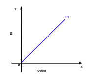 |
Inverted parabola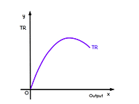 |
| Demand curve-price line | A straight line parallel to the “x” axis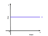 |
Downward sloping straight line. It is the AR curve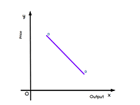 |
| Marginal Revenue | MR will be same for all the units of output. MR will be equal to price(P = MR). It will be a straight line parallel to “x” axis. It is same as the demand curve.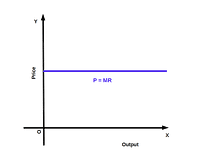 |
As the output increases MR decreases. MR curve will be under the demand curve or the AR curve.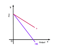 |
| Average Revenue | For each unit of output ( P = MR = AR). AR curve is parallel to “x” axis.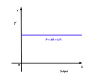 |
As output increases AR decreases. It is also the demand curve of the firm.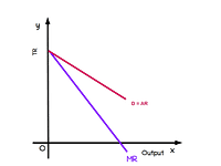 |
Short-run equilibrium of monopoly Profit maximization is the main objective of every monopoly firm. Now we can discuss this profit maximising behaviour to determine the quantity produced and the price at which it is sold. Here the assumption is that the entire quantity produced is put up for sale without maintaining stocks. The monopoly firm maximises profit under two different situations.
- The simple case of zero cost, and
- In case of positive costs.
1. The simple case of zero cost This is a monopoly situation in which the cost of production is zero (TC = 0). It is a very rare case. Suppose an individual has a mineral water well in his plot in a village far away from other villages. All inhabitants of that village draw water from this well. The owner of the well does not allow any villager to take water from this well without paying for it. So the owner of this well is a monopolist. Those who need water can draw it from the well with the permission of the owner. There is no cost of production for water. We can now explain the price and output determination under monopoly in which cost of production is zero.
Monopoly market reaches equilibrium when profit is maximum. Profit (x) is the difference between total revenue and total cost. Then, the Profit of the monopoly with zero cost isπ = TR – TC = TR – 0 = TR
 Profit : π = TR – TC ( TR = AR × q )
= OP × Oq = area OqaP
Profit will not be maximised before and after Oq. When profit is maximum MR is zero. In a monopoly market with zero cost at output q, MR is zero and TR is maximum.
The equilibrium quantity of a monopoly with zero cost will be half of the market demand when price is zero.
In the demand function q = 20 – 2P. When price is zero, output is 20 units.
ie.,q = 20 – 2P = 20 – 2 × 0 = 20
So equilibrium quantity is 10 units which is half of 20.
Price at maximum profit is 5.
ie, P = 10 – .5q = 10 – .5 ×10
= 10 – 5 = 5
Profit, π = TR – TC = Pq – TC
= 5 × 10 – 0 = 50
Profit : π = TR – TC ( TR = AR × q )
= OP × Oq = area OqaP
Profit will not be maximised before and after Oq. When profit is maximum MR is zero. In a monopoly market with zero cost at output q, MR is zero and TR is maximum.
The equilibrium quantity of a monopoly with zero cost will be half of the market demand when price is zero.
In the demand function q = 20 – 2P. When price is zero, output is 20 units.
ie.,q = 20 – 2P = 20 – 2 × 0 = 20
So equilibrium quantity is 10 units which is half of 20.
Price at maximum profit is 5.
ie, P = 10 – .5q = 10 – .5 ×10
= 10 – 5 = 5
Profit, π = TR – TC = Pq – TC
= 5 × 10 – 0 = 50
Comparing monopoly with Perfect Competition If we compare a zero cost monopoly market with a zero cost perfectly competitive market, price under perfectly competitive market will be low, and output would be more and hence profit will be less. Let us see how this happens.
In a perfectly competitive market there will be infinite number of mineral water well owners with zero cost. Suppose one of them tries to increase profit by reducing price and selling more. Then the consumers will draw water from the low price firm. With the expectation of selling more other firms also decrease the price. Thus price goes on decreasing till it becomes zero. When price is decreased, they can sell more. This increases market supply. Perfect competition provides less price and more quantity than a monopoly market. Profit will be highest in the monopoly market. Monopolist earns abnormal profit. But in perfect competition, firms earn only normal profit. As the price is low, profit also will be low.2. In case of positive costs The equilibrium of monopoly with Positive cost can be analysed into two methods. They are:
- (a) TR-TC approach
- (b) MR~MC approach
(a) Total Revenue — Total Cost Approach A firm reaches equilibrium when profit is maximum. We know that π = TR – TC. Under Total Revenue – Total Cost approach, a monopoly firm reaches equilibrium when total revenue is higher than total cost, and the difference between the two is maximum. i.e,
- TR must be more than TC, and
- Difference between TR and TC must be the maximum
 Between output level q1 and q2 TR is higher than TC. Then profit curve is in the positive region. When quantity of output is q the difference petween TR and TC is at maximum.
At quantity q, the profit curve increases and reaches its maximum. Therefore, q is the equilibrium quantity of output at maximum profit of a monopoly with positive cost.
Between output level q1 and q2 TR is higher than TC. Then profit curve is in the positive region. When quantity of output is q the difference petween TR and TC is at maximum.
At quantity q, the profit curve increases and reaches its maximum. Therefore, q is the equilibrium quantity of output at maximum profit of a monopoly with positive cost.
| Table 6.4 | ||
| q | P | TC |
|---|---|---|
| 0 | 10 | 5 |
| 1 | 9 | 12 |
| 2 | 8 | 16 |
| 3 | 7 | 17 |
| 4 | 6 | 19 |
| 5 | 5.5 | 20 |
| 6 | 4 | 20 |
| 7 | 3 | 21 |
| 8 | 2.5 | 23 |
| 9 | 2 | 25 |
- (1) Find the TR and profit at different output levels.
- (2) What is the equilibrium quantity?
- (3) What is the equilibrium price?
- (4) What is the profit at equilibrium quantity?
- (5) Find TR and TC, when profit is maximum.
- (1)
Table 6.5 q P TR TC π 0 10 – 5 -5 1 9 9 12 -3 2 8 16 16 0 3 7 21 17 4 4 6 24 19 5 5 5.5 27.5 20 7.5 6 4 24 20 4 7 3 21 21 0 8 2.5 20 23 -3 9 2 18 25 -7 - (2) 5 units
- (3) ₹ 5.5
- (4) ₹ 7.5
- (5) TR = ₹ 27.5 TC = ₹ 20
(b) Marginal Revenue – Marginal Cost Approach Under MR- MC approach a monopoly firm attains equilibrium when two conditions are fulfilled. They are:
- Marginal revenue and Marginal cost should be equal (MR = MC)
- MC curve should cut MR curve from below.
 π = TR – TC = AR × q – AC × q
= OP × Oq – OT × Oq
= OPRq – OTSq
= TPRS, the shaded area, is the maximum profit.
π = TR – TC = AR × q – AC × q
= OP × Oq – OT × Oq
= OPRq – OTSq
= TPRS, the shaded area, is the maximum profit.
| Table 6.6 | ||
| q | P | TC |
|---|---|---|
| 0 | 12 | 10 |
| 1 | 11 | 17 |
| 2 | 10 | 18 |
| 3 | 9 | 22 |
| 4 | 8 | 27 |
| 5 | 7 | 38 |
- (1) Find TR, AR, MR, MC, AC and profit at different levels of output.
- (2) What is the equilibrium quantity ? Why ?
- (3) What is the equilibrium price ?
- (4) What is the profit at equilibrium quantity ?
- (5) What is the MR and MC at equilibrium quantity ?
- (6) What is the AR at equilibrium quantity ?
- (7) What are TR and TC at maximum profit ?
| Table 6.7 | ||||||||
|---|---|---|---|---|---|---|---|---|
| q | P | TR | TC | MR | MC | AR | AC | Profit |
| 0 | 12 | 0 | 10 | – | – | – | – | -10 |
| 1 | 11 | 11 | 17 | 11 | 7 | 11 | 17 | -6 |
| 2 | 10 | 20 | 18 | 9 | 1 | 10 | 9 | 2 |
| 3 | 9 | 27 | 22 | 7 | 4 | 9 | 7.33 | 5 |
| 4 | 8 | 32 | 27 | 5 | 5 | 8 | 6.75 | 5 |
| 5 | 7 | 35 | 38 | 3 | 11 | 7 | 7.6 | -3 |
Comparison of Monopoly with Perfect Competition Equilibrium quantity under perfect competition will be more than the equilibrium quantity of monopoly market. As the monopolist can sell less quantity of output at high price, price in monopoly market will always be higher than the price under perfect competition. Moreover, profit of monopoly firm will always be much higher than the profit under perfectly competitive firm.
In the long run Ina perfectly competitive market, some firms may earn abnormal profits and some others may incur loss in the short-run. If any one firm makes abnormal profit, new firms will enter that industry, and abnormal profit will cease to exist. But if any one firm function’ under loss, that firm will have to stop production and leave. So in perfectly competitive market all firms will earn normal profit only, in the long run.
As there is no entry into monopoly market, the: monopolist makes abnormal profits both in the short run and long run.Critical Views on Monopoly There are several criticisms levelled against monopoly firms which are given below:
- Monopoly firms charge higher price for goods.
- Monopoly firms solely benefit themselves, at the cost of consumers.
- Monopoly firms receive higher profit even in the long run.
- Consumers get lesser quantity of output for which they have to pay more.
| Table 6.8 | |
| Perfect Competition | Monopoly |
|---|---|
| The producer is the price taker | The producer is the price maker |
| Large number of firms | Single seller |
| Homogeneous product | No substitutes |
| Free entry | Entry is declined |
| Horizontal demand curve | Downward sloping demand curve |
| Perfectly elastic demand | Less elastic demand |
| TR curve is linear | TR curve is an inverted parabola |
Monopolistic Competition Pure monopoly and perfect competition are rare in practice. The markets that we come across in our daily life have characteristics of competition and monopoly. Such a 3 market is monopolistic competition.
Monopolistic competition, as the name implies, is a blend of monopoly and competition. It is a market situation characterised by fairly large number of firms producing and selling differentiated goods and services. For example, the firms which produce consumer goods such as toilet soaps, shampoos, biscuits, tooth-paste, etc. It was Edward Chamberlin who popularised monopolistic competition through his book ‘The Theory of Monopolistic Competition’ in 1956.Features of Monopolistic Competition
- Fairly large number of buyers and sellers but their number is less than under perfect competition.
- There will be product differentiation, The product of each firm is known by a brand name. Products of each firm will be different from those of other firms in quality, colour, smell, taste, etc.
- Firms can freely enter and exit from the market
- There will be selling costs like the expenses for advertisement, propaganda, coupons, gifts and other selling strategy
- Differences in price. Because of product differentiation prices also will be different.
Demand Curve under Monopolistic Competition Under monopolistic competition, the demand curve will slope down-wards from left to right. So producers can sell more by decreasing price. The demand curve would be flatter than that of monopoly. It signifies a high price elasticity of demand. Here the demand curve is same as. AR curve.
Equilibrium under Monopolistic Competition There is a minor difference in the Conditions of price and output determination (Equilibrium) in the short- run and long-run under monopolistic competition. Accordingly, the equilibrium under monopolistic competition can be discussed under two heads:
- (1) Short-run equilibrium and
- (2) Long-run equilibrium
Short-run Equilibrium A firm under monopolistic competition attains equilibrium in the short run when it satisfies two conditions:
- (1) MR=MC
- (2) MC curve should be rising. MC curve should cut MR curve from below.
 Comparing with perfect competition the equilibrium quantity is less in monopolistic competition and the equilibrium price will be high. While comparing with monopoly under monopolistic competition the equilibrium quantity will be high and equilibrium price will be less.
Long run Equilibrium Long run equilibrium under, monopolistic competition is called group equilibrium. Firms in the industry have complete freedom to enter and exit the monopolistic market. In the short run, if any firm earns profits, new firms will enter the industry. Consequently output expands and prices in the market fall till profit becomes zero. Now there is no attraction for the new firms to enter. On the contrary, if any firm incurs loss in the short run, that firm will stop production and exit the market. Now there will be a fall in output leading to higher price. Entry or exit would stop once profit becomes zero. This would act as the long run equilibrium. Under monopolistic competition, all firms earn normal profits in the long run.
Oligopoly Oligopoly is an important form of imperfect competition. The word Oligopoly is derived from the words ‘Oligo’ and ‘poly’ which means a few and sellers respectively. So oligopoly means a few sellers. Oligopoly is a market situation in which there are a few firms that produce homogeneous or differentiated goods and compete with one another. Firms manufacturing car, motor cycle, scooter, mobile phone, etc., are examples of oligopoly firms.
Features of Oligopoly
- A few sellers: The number of producers or sellers will be small in oligopoly.
- Homogeneous or differentiated product: Products sold in oligopoly will be either homogeneous, like cooking gas, steel, petrol, etc., or differentiated, like car, motor cycle, scooter, etc.
- Free entry and exit: Firms can freely enter and exit from the market.
- Selling cost: Large amounts are spent on advertisements and boosting sale.
- Interdependence between firms: As the number of firms in oligopoly is small, there is interdependence among them. Decision taken by one firm affects other firms.
- Indeterminateness of demand curve: The demand curve under oligopoly is indeterminate. It may be high elasticity or low elasticity demand.
- Price leadership: Sometimes in an oligopoly, one firm may emerge as a leader and determine the price.
Duopoly Duopoly is a special case of oligopoly in which there are only two sellers or producers.
Here the assumption is that product sold by the two firms is homogeneous and there is no close substitutes. In such a situation output decisions of any one firm will affect the market price, quantity sold by other firms and their total revenues. It is to be expected that other firms would react to safeguard their profits. This would be through taking new decisions about quantity and price. Economists have formed different models which examine the behaviour of duopoly firms.- 1. Collusive Duopoly model
- 2. Cournot Duopoly model
- 3. Kinked demand curve model
1. Collusive Duopoly Model Collusive Duopoly is one model of duopoly. In this model, the two firms do not compete with each other but collude together and try to maximise their profit. These two firms produce their products in different factories, but they behave like a single monopoly.
2. Cournot’s Duopoly Model
Augustine Cournot, a French economist in 1838, devéloped a model which is known as Cournot’s duopoly model. Cournot explains his duopoly model with an example of two production units.
Assumptions
- (1) There are two firms or producers.
- (2) Both firms sell identical products.
- (3) Cost of production is zero.
- (4) The demand curves of the firms are linear.
- (5) Each firm assumes that the firm will keep its output constant.
- (6) The objective of the firms is to maximise profit.
Conditions of duopoly equilibrium
- In duopoly, as cost of production is zero, MR = MC = 0.
- At the last stage, supply of both firms should be equal. Supply of each producer should be one-third of total market demand in which the price is zero.
| Table 6.9 | |||
|---|---|---|---|
| Stages | Firms | Quantity supplied | Answers |
| 1 | B A |
0 \(\mathbf{\frac{1}{2}}\) × 20 = \(\mathbf{\frac{20}{2}}\) |
0 10 |
| 2 | B A |
\(\mathbf{\frac{1}{2}}\)\(\biggl(\mathbf{20-\frac{1}{2}× 20} \biggr)\) = \(\mathbf{\frac{20}{2}}\) – \(\mathbf{\frac{20}{4}}\) \(\mathbf{\frac{1}{2}}\) \(\biggl(\mathbf{20-\frac{1}{2} \biggl(20-\frac{1}{2}× 20} \biggr)\biggr)\) = \(\mathbf{\frac{20}{2}}\) – \(\mathbf{\frac{20}{4}}\) + \(\mathbf{\frac{20}{8}}\) |
5 7.5 |
| 3 | B | \(\mathbf{\frac{1}{2}}\) \(\biggl(\mathbf{20-\frac{1}{2}} \biggl(\mathbf{20-\frac{1}{2} \biggl(20-\frac{1}{2}× 20} \biggr)\biggr)\biggr)\) = \(\mathbf{\frac{20}{2}}\) – \(\mathbf{\frac{20}{4}}\) + \(\mathbf{\frac{20}{8}}\) – \(\mathbf{\frac{20}{16}}\) and so on |
6.25 |
| . . . |
. . . |
. . . |
. . . |
The equilibrium price Since, P = 10 – .5q
= 10 – .5 × \(\frac{40}{3}\) (since q = \(\frac{40}{3}\)) = 10 – \(\frac{20}{3}\) = \(\frac{30}{3}\) – \(\frac{20}{3}\) = \(\frac{10}{3}\) = ₹ 3.33 ( This is lower than the price under monopoly but higher than under perfect competition). The profit of firm A is π = pq – TC = \(\frac{10}{3}\) × \(\frac{10}{3}\) – 0 = 22.22 The profit of firm B is also 22.22 and the profit of A and B in the industry is 44.44.3. Kinked Demand Curve Model

The concept of kinked demand curve under oligopoly was developed by Paul M Sweezy. Kinked demand curve explains the peculiar nature of demand under oligopoly conditions. This model explains price rigidity. It refers to the tendency of price to remain steady without change. When one firm increases price to get more income and profit, the second firm does not follow, there will be a huge fall in the income and profit of the firm that had increased the price. The demand of the firm will be relatively elastic. If any firm wants to sell more output and increase profits by reducing price, the other firm also will imitate it. The continuous price reduction will lead to big loss. Therefore, decreasing price is irrational. Here, its demand curve will be relatively inelastic. Price would be more rigid in this model than in a perfectly competitive market.
| Table 6.10 | ||||
|---|---|---|---|---|
| Features | Perfect Competition | Monopoly | Monopolistic Competition | Oligopoly |
| 1. Number of firms | Large number | One | Fairly large | A few |
| 2. Natur of product | Homogeneous | Homogeneous (No close Substitute) |
Product diffrentiation | Homogeneous or Difrentiated |
| 3. Freedom of entry | Yes | No | Yes | Yes |
| 4. Price | Same price | Very high | High | High |
| 5. Selling cost | No | No | Yes | Yes |
| 6. Elasticity | Perfect elastic demand | Less elastic demand | High elastic demand | Various forms |
| 7. Demand curve | Horizontal | Downward sloping less flatter | Downward sloping more flatter | Cannot determinate, kinked form |
![]()
0 Comments