Plus Two Economics-Chapter 5
Chapter 5:-


Introduction In a free market economy, prices of goods and services are determined by demand and supply. The process of determining prices of goods and services by demand and supply is called price mechanism. Price mechanism is an important feature of capitalist economy. We shall discuss how demand and supply determine price.
Equilibrium, Excess Demand, Excess Supply Equilibrium means balance or equal. That is, there is no tendency to move in either direction. Equilibrium is defined as a situation in which the objectives of all firms (profits) and consumers (preferences) are satisfied and the market is cleared. At equilibrium point the quantity of goods sold by all the firms and the quantity of goods bought by all the consumers are equal, i.e., market demand will be equal to market supply at equilibrium.
The price at which demand and supply are equal is known as equilibrium price. The quantity demanded and supplied will be equal at the equilibrium price. When the price is very high buyers are not willing to buy. When the price is low producers are not willing to sell. So the firms are forced to reduce price and the buyers are forced to give high price. In this way equilibrium price is determined by demand and supply. The quantity of goods sold and bought at equilibrium price is called equilibrium quantity. We have studied that demand and supply are the functions of price. Therefore equilibrium conditions can be written as qd (p*) = qs (p*) where qd (p*) is market demand and qs (p*) is the market supply then p*, q* are equilibrium price and equilibrium quantity respectively. In the above Diagram DD is the market demand curve and SS is the market supply curve. DD and SS intersect at point E. This is the market equilibrium where DD = SS. P* is the equilibrium price and q* is the equilibrium quantity.
The situation in which market demand is higher than market supply at a given price is called excess demand.
The situation in which market supply is higher than market demand at a given price is called excess supply.
Therefore, in a perfectly competitive market, equilibrium can be defined as a situation in which there is no excess demand and no excess supply.
In the above Diagram DD is the market demand curve and SS is the market supply curve. DD and SS intersect at point E. This is the market equilibrium where DD = SS. P* is the equilibrium price and q* is the equilibrium quantity.
The situation in which market demand is higher than market supply at a given price is called excess demand.
The situation in which market supply is higher than market demand at a given price is called excess supply.
Therefore, in a perfectly competitive market, equilibrium can be defined as a situation in which there is no excess demand and no excess supply.

Out of Equilibrium Behaviour
Whenever there is imbalance or disequilibria in the perfectly competitive market, an invisible hand will work, according to Adam Smith (1723-1790). In case of ‘excess demand’, this invisible hand will increase the price. Likewise in case of ‘excess supply’, invisible hand will lower the price. By following this Process, equilibrium is attained in the market.
| Table 5.1 | |||
|---|---|---|---|
| Price | Demand | Supply | Condition |
| 10 | 800 | 400 | 400 – Excess Demand (D > S) |
| 20 | 600 | 600 | Equilibrium (D = S) |
| 30 | 500 | 700 | 200 – Excess Supply (S > D) |
| Table 5.2 | |||
|---|---|---|---|
| Price | Demand | Supply | Condition |
| 10 | 500 | 100 | 400 – Excess Demand (D > S) |
| 20 | 400 | 200 | 200 – Excess Demand (D > S) |
| 30 | 300 | 300 | Equilibrium (D = S) |
| 40 | 200 | 400 | 200 – Excess Supply (S > D) |
| 50 | 100 | 500 | 400 – Excess Supply (S > D) |

| Table 5.3 | ||
|---|---|---|
| Price | Demand | Supply |
| 10 | 1000 | 300 |
| 20 | 900 | 400 |
| 30 | 700 | 500 |
| 40 | 650 | 650 |
| 50 | 600 | 800 |
| 60 | 400 | 1000 |
- (1) Find excess demand and excess supply at different prices.
- (2) What is the equilibrium price?
- (3) What is the equilibrium quantity?
- (1) 700, 500 and 200 are the excess demand at prices 10, 20, and 30 respectively and 200 and 600 are the excess supply at prices 50 and 60 respectively.
- (2) ₹ 40
- (3) 650 kg
Market Equilibrium when there is Fixed Number of Firms In a market with number of firms fixed — (Here we assume that there is no entry and exit of firms) the determination of market equilibrium can be explained as follows. When the number of firms is fixed, as a result of the forces of demand and supply the market attains equilibrium. That is, when price rises demand falls, and when price falls demand rises, Similarly, when price rises, supply rises and when price falls supply falls. These two opposite forces act together and determine the Price of goods and services. It can be explained with the help of Diagram given below.
 Demand and supply are marked on the x-axis and price is marked on the y-axis. DD is the market demand curve and SS is the market supply curve. At point E the quantity of demand and quantity of supply are equal and demand curve and supply curve intersect each other and reaches equilibrium. Here the quantity of demand and supply are q* and the price is p*. Therefore, p* is the equilibrium price and q* is the equilibrium quantity and there is neither excess demand nor excess supply.
Now, suppose the price is p1. Then quantity of supply is q1, the demand is q4. At price p1, q1 q4 is excess demand. This makes the price to rise from p1 to p*. Similarly, let us suppose price is p2. Then quantity of demand is q2, the quantity of supply is q3. At price p2, q2 q3 is the excess supply. This causes price to fall from P2 to p*. At price p* excess demand and excess supply are zero. In this Way the demand and supply together make the market equilibrium under fixed number of firms.
Suppose Price of a commodity is₹ 10, market supply is 100 kg and market demand is 700 kg. This is shown in the below Graph. So excess demand is 600 kg. This excess demand increases the price. If market price is ₹ 60 market demand is 200 kg. and market supply is 600 kg. Then excess supply is 400 kg. This excess supply leads to a fall in market price. If market price is ₹ 40, market demand and market supply would be 400 kg. Here excess demand and excess supply is zero. Therefore, from the below graph we can conclude that, equilibrium price is ₹ 40, and equilibrium quantity is 400 kg.
If price is above ₹ 40, there will be excess supply; if it is below ₹ 40 there will be excess demand.
Demand and supply are marked on the x-axis and price is marked on the y-axis. DD is the market demand curve and SS is the market supply curve. At point E the quantity of demand and quantity of supply are equal and demand curve and supply curve intersect each other and reaches equilibrium. Here the quantity of demand and supply are q* and the price is p*. Therefore, p* is the equilibrium price and q* is the equilibrium quantity and there is neither excess demand nor excess supply.
Now, suppose the price is p1. Then quantity of supply is q1, the demand is q4. At price p1, q1 q4 is excess demand. This makes the price to rise from p1 to p*. Similarly, let us suppose price is p2. Then quantity of demand is q2, the quantity of supply is q3. At price p2, q2 q3 is the excess supply. This causes price to fall from P2 to p*. At price p* excess demand and excess supply are zero. In this Way the demand and supply together make the market equilibrium under fixed number of firms.
Suppose Price of a commodity is₹ 10, market supply is 100 kg and market demand is 700 kg. This is shown in the below Graph. So excess demand is 600 kg. This excess demand increases the price. If market price is ₹ 60 market demand is 200 kg. and market supply is 600 kg. Then excess supply is 400 kg. This excess supply leads to a fall in market price. If market price is ₹ 40, market demand and market supply would be 400 kg. Here excess demand and excess supply is zero. Therefore, from the below graph we can conclude that, equilibrium price is ₹ 40, and equilibrium quantity is 400 kg.
If price is above ₹ 40, there will be excess supply; if it is below ₹ 40 there will be excess demand.

Method of determination of equilibrium price and quantity using equation If the demand function and supply function are known, equilibrium price and quantity can be determined. Look at the below given problem.
If qd = 200 – P is demand function and qs = 120 + P is the supply function at equilibrium. qd = qs 120 + P= 200 – P; Solve for P P + P =200-120 2P = 80 P = \(\frac{80}{2}\) = 40 is the equilibrium price. The value of P can be substituted in demand function or supply function. qd = 200 – P = 200 – 40 = 160 or qs = 120 + P= 120 + 40 = 160 qd = qs = 160 unit is the equilibrium quantity. If market price is less than equilibrium price it will be excess demand. For example, suppose market price P = ₹ 25. qd = 200 – P = 200 – 25 = 175 qs = 120 + P = 120 + 25 = 145Excess demand ED = qd – qs = 175 – 145 = 30
If market price is more than equilibrium price there will be excess supply in the market. For example, suppose P= ₹ 45, then qd = 200 – P = 200 – 45 = 155 qs = 120 + P = 120 + 45 = 165Excess supply ES = qs – qd = 165 – 155 = 10
If qd = 100 – P is the market demand curve and qs = 20 +P is the market supply curve, find Equilibrium price and quantity. At equilibrium, qs = qd 20 + P = 100 – P P + P = 100 – 20 2P = 80 P = \(\frac{80}{2}\) = 40 Equilibrium demand: qd = 100-P = 100 – 40 = 60 Equilibrium supply: qs = 20 + P = 20 + 40 = 60Wage Determination in Labour Market
We have seen how the price of a product is determined under perfectly competitive conditions using demand-supply analysis. Now, let us use the same demand-supply analysis to explain wage determination under perfectly competitive conditions.
There is an important point of difference between market for goods and market for labour. In the case of goods, demand mostly comes from consumers and supply comes from firms. But in the case of labour, demand comes from firms and supply comes from households.How much labour will a firm demand ? A firm under perfectly competitive conditions aims at profit maximisation. Such a firm will employ (demand) labour up to the point where the additional cost of employing the last unit of labour is equal to the additional benefit that it earns from it. The additional cost is wage (W) and the additional benefit is the marginal revenue product of labour (MRPL). MRPL is arrived at by multiplying marginal revenue by the marginal product of labour.
Therefore, a firm will demand labour up to the point whereW = MRPL
The demand curve for labour will be downward sloping. This is due to the declining marginal productivity of labour caused by the operation of the law of diminishing returns. More labour will be demanded only at lower wage rates.
What about the supply of labour ? Supply of labour comes from households. Wage rate – labour supply relationship is complex. From an individual labourer’s point of view the supply curve of labour can be backward sloping. This is because, at high wage rates, workers may prefer leisure to work. This may reduce the supply of labour at high wage rates. But this is applicable only in the case of individual supply and not market supply. Market supply of labour will increase at higher wage rates. This is because higher wages will attract more workers. Therefore, market supply curve of labour will be upward sloping to the right.
Equilibrium wage rate will be determined at the point where the downward sloping demand curve for labour intersects the upward sloping supply curve of labour. This is shown in the following diagram. OW is the equilibrium wage rate.
Shifts in Demand and Supply We have seen that equilibrium price is the one at which the quantity demanded equals quantity supplied, assuming factors other than the price of the commodity remaining constant. So whenever there is shift in demand or shift in supply, new equilibrium emerges in price and quantity. We discuss the effects of shifts (changes) in demand and supply on equilibrium price and quantity under following heads.
I. Shifts (changes) in demand while supply remains the same. I. Shifts (changes) in supply while demand remains the same. III. Simultaneous shifts (changes) in demand and supply- (a) Simultaneous increase in demand and supply
- (b) Simultaneous decrease in demand and supply
I Shifts in Demand Demand curve shifts due to the changes in non-price factors like consumer’s income, prices of other commodities and tastes and preferences of the consumer. Market demand curve shifts to the right due to the favourable change in non-price factors. Market demand curve shifts to the left due to the unfavourable changes in non-price factors. In such cases, market supply curve remains unchanged.
(a) The demand curve shifts rightward and supply remains the same Market demand curve shifts towards the right in favourable circumstances like increase in the income of the consumer in case of normal goods, decrease in the income of the consumer in case of inferior goods; increase in price of substitute goods, decrease of price of complementary goods, and increase in the number of consumers.
In the below Diagram, DD is the market demand curve and SS is the market supply curve. E is the initial equilibrium where the market demand and market supply intersect, P is the equilibrium price and q is the equilibrium quantity. DD shifts rightward as D1 D1 due to the favourable changes in non-price factors. Now, at price P, market demand is q’ and supply is the same q. The demand is higher than supply. Then excess demand is q q’. So some consumers are willing to pay higher prices. As a result equilibrium price increases to P1 . E1 is the new equilibrium where the new market demand curve D1 D1 and the market supply curve SS intersect. The new equilibrium price is P1 . New equilibrium quantity is q1 .
(b) The demand curve shifts left-ward and supply remains the same Market demand curve shifts towards the left in unfavourable circumstances like decrease in income of the consumer in case of normal goods, increase in the income of the consumer in case inferior goods, decrease in the price of substitute goods and decrease in the number of consumers.
 Demand curve DD shifts to D2D2 due to unfavourable changes in non-price factors. Now at price P market demand is q’ and market supply q. Compared to market demand, market
supply is high. q’q is the excess supply. So the producers are ready to cut the price. Price falls to P2. E2 is the new equilibrium point. Where the new market demand curve D2D2 and the market supply curve SS intersect each other. The new equilibrium price is P2 and new equilibrium quantity is q2. When the demand curve shifts leftward and supply remains the Same, the equilibrium price and quantity decrease.
Demand curve DD shifts to D2D2 due to unfavourable changes in non-price factors. Now at price P market demand is q’ and market supply q. Compared to market demand, market
supply is high. q’q is the excess supply. So the producers are ready to cut the price. Price falls to P2. E2 is the new equilibrium point. Where the new market demand curve D2D2 and the market supply curve SS intersect each other. The new equilibrium price is P2 and new equilibrium quantity is q2. When the demand curve shifts leftward and supply remains the Same, the equilibrium price and quantity decrease.
II Shifts in Supply Market supply curve shifts due to the changes in non-price factors like price of inputs, technology, unit tax, etc. Market supply curve shifts towards the right due to favourable change in non-price factors. Market supply curve shifts towards the left due to unfavourable changes in non-price factors. In such cases market demand curve-remains unchanged.
(a) The supply curve shifts rightward and demand remains the same Market supply curve shifts to the right when the price of inputs decreases, taxes come down, technology improves and the number of firms increases.
 Supply is higher than demand. On account of excess supply q q’ producers decrease the price. At point E1 the new market supply curve S1S1 and market demand curve, DD
intersect. The new equilibrium price is P1. New equilibrium quantity is q1.
When market supply shifts rightward and the demand remains the same, equilibrium price decreases and equilibrium quantity increases.
Supply is higher than demand. On account of excess supply q q’ producers decrease the price. At point E1 the new market supply curve S1S1 and market demand curve, DD
intersect. The new equilibrium price is P1. New equilibrium quantity is q1.
When market supply shifts rightward and the demand remains the same, equilibrium price decreases and equilibrium quantity increases.
(b) The supply curve shifts leftward and demand remains the same Due to increase in price of inputs, tax increase, use of outdated technology and decrease in the number of producers market supply curve shifts to left.
 In the above Diagram market demand curve DD and market supply curve SS intersect at equilibrium point E. Equilibrium price is P and quantity is q. On account of adverse changes in non-price factors market supply curve SS shifts to the left as S2S2. Now at price P market supply is q’ and market demand curve remains the same as q. Supply is less compared to demand. Because of excess demand q’q consumers are willing to pay higher price. At point E2 the new market supply curve S2S2 and the market demand curve DD intersect. The new equilibrium price is P2. New equilibrium quantity is q2.
When market supply shifts leftward and the demand remains the same equilibrium price increases and equilibrium quantity decreases.
In the above Diagram market demand curve DD and market supply curve SS intersect at equilibrium point E. Equilibrium price is P and quantity is q. On account of adverse changes in non-price factors market supply curve SS shifts to the left as S2S2. Now at price P market supply is q’ and market demand curve remains the same as q. Supply is less compared to demand. Because of excess demand q’q consumers are willing to pay higher price. At point E2 the new market supply curve S2S2 and the market demand curve DD intersect. The new equilibrium price is P2. New equilibrium quantity is q2.
When market supply shifts leftward and the demand remains the same equilibrium price increases and equilibrium quantity decreases.
III Simultaneous Shifts of Demand and Supply The simultaneous shifts can happen in four possible ways.
- Both demand and supply curves shift rightwards.
- Both demand and supply curves shift leftwards.
- Demand curve shifts rightward and supply curve shifts leftward.
- Demand curve shifts leftward and supply curve shifts rightward.
| Table 5.4 | |||
|---|---|---|---|
| Shift in Demand | Shift in Supply | Quantity | Price |
| Rightward | Rightward | Increases | May increase, decrease or remain unchanged |
| Leftward | Leftward | Decreases | May increase, decrease or remain unchanged |
| Rightward | Leftward | May increase, decrease or remain unchanged | Increases |
| Leftward | Rightward | May increase, decrease or remain unchanged | Decreases |
 If rate of increase in demand is less than the rate of increase in supply, equilibrium price will come down. This is shown in below diagram Change in D1D1 is less than that of S1S1.
 If the rate of increase in demand and supply is same the equilibrium price remains unchanged. It is shown in the below given Diagram.
Both demand and supply curves shift rightwards.
Both demand and supply curves shift leftwards.

Both demand and supply curves shift opposit direction.
Market Equilibrium: Free Entry and Exit Now we shall discuss how firms under free entry and exit attain market equilibrium. In this market new firms can freely enter the industry and existing firm can leave the industry at any time.
Free entry and exit imply that no firm earns super normal profit or incurs loss at equilibrium. All firms earn normal profits. If there is super normal profit in an industry, new firms enter. The entry of new firms increases supply. As a result, the supply curve shifts to the right and price comes down and super normal profit disappears. Similarly, when existing firms incur loss, they stop production and leave the industry. When they leave, supply decreases and the supply curve shifts to the left. As a result price increases and firms get normal profit. Firms earn normal profit when price is equal to minimum average cost. So where there is free entry and exit, equilibrium price will be equal to the minimum point of average cost, i.e.,P = Minimum AC
In other words, when price is more than minimum AC, new firms will enter the market, and when price is less than minimum AC, some existing firms stop production and leave the market. Therefore, in perfect competition price will always be the minimum of Average Cost.
 In this situation, supply will be perfectly elastic. Therefore, the quantity of output supplied at minimum AC is determined by the market demand at that price. In the above Diagram the demand curve DD intersects P0 = min AC line at point E. P0 is the equilibrium price and q0 is the equilibrium quantity.
P0, is equal to the minimum of AC. Total supply and total demand are equal (q0) at P0 price.
If market price, P0 = min AC, q0 is market demand, qf is the supply of a firm, n0 is the number of firms, at price P0 the number of equilibrium firms in the market will be
In this situation, supply will be perfectly elastic. Therefore, the quantity of output supplied at minimum AC is determined by the market demand at that price. In the above Diagram the demand curve DD intersects P0 = min AC line at point E. P0 is the equilibrium price and q0 is the equilibrium quantity.
P0, is equal to the minimum of AC. Total supply and total demand are equal (q0) at P0 price.
If market price, P0 = min AC, q0 is market demand, qf is the supply of a firm, n0 is the number of firms, at price P0 the number of equilibrium firms in the market will be
\( n_{0} = \frac{q_{0}}{q_{f}}\)
Suppose, market demand function q0D = 200 – P, supply function qfs = 10 + P and market price P0 = min AC = 20. Market demand:
qD = q0 = 200 – P = 200 – 20 = 180 (P = P0 = 20) Supply of one firm at P0 = 20: qfs 10 + P = 10 + 20 = 30 Equilibrium number of firms n0 = \(\frac{q_{0}}{q_{f}}\) = \(\frac{180}{30}\) = 6 In a market with free exit and entry the supply curve of a firm is qfs 20 + P, demand curve is qD = 100 – P and minimum AC is ₹ 10.- Find the equilibrium price.
- What is equilibrium demand?
- What is the supply of a firm?
- Find number of firms in the market.
- What is the total supply?
- Equilibrium market price is ₹ 10
- qD = q0 = 100 – P = 100 – 10 = 90
- qfs 20 + P = 20 + 10 = 30
- \( n_{0} = \frac{q_{0}}{q_{f}}\) = \(\frac{90}{30}\) = 3
- Total supply = qfs × n0 = 30 × 3 = 90
Shifts in Demand Curve We can examine the effect of shifts in demand curve on equilibrium quantity and number of firms under free entry and exit. The increase in demand for some reasons shifts the demand curve from DD to D1D1 as shown in the below Diagram.

- (1) If the demand curve shifts to right, equilibrium quantity and equilibrium number of firms will increase, but equilibrium price will remain the same in the market where there is free entry and exit.
- (2) When demand curve shifts to left equilibrium price remains the same and equilibrium quantity and number of firms decrease.

Applications Now we can discuss the impact of government intervention in price determination in demand-supply analysis. Price ceiling and floor price are examples of government intervention in price determination. The government fixes price ceiling for some goods to protect consumers. Similarly, price floor is declared for some goods to protect producers.
Price Ceiling Price ceiling is the upper limit on the price of goods and services imposed by the government to protect the interest of consumers. It is generally imposed on essential items. For example, in India, prices of essential drugs and prices of food grains, sugar, kerosene, etc., are fixed by the government, below market – determined price. The price ceiling will always be less than equilibrium price.
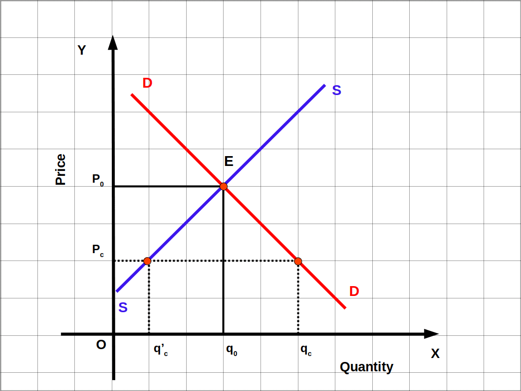
- long queue in the ration shops,
- the consumers get less than what they want through the ration shops. Some consumers are willing to pay higher price due to excess demand. This may result in the creation of black market.
Floor Price Price floor or support price is the minimum price of goods and services imposed by the government to protect the interest of producers. When the price determined by the forces of demand-supply is very low, the producers suffer much loss. Then the government intervenes in the market and declares price floor. In India the declaration of price floor for paddy and coconut, and minimum wages for workers are examples.
 The price floor imposed by the government will be more than equilibrium price. We can explain the impact of floor price in the market with the help of above Diagram. Demand curve DD and supply curve
SS intersect at the point E. In market equilibrium price. is P0. Equilibrium quantity is q0. The price floor declared by the government to protect the interests of the farmers producers is Pf which is higher than the market price. At Pf market demand is qf and market supply is qf. At Pf supply is more than demand. This causes excess supply. Here excess supply is qf‘qf. The surplus commodity due to government’s floor price declaration is collected by the government at Pf price. The product thus stocked by the government is sold when market price rises. If this surplus commodity is not collected by the government market price will go down.
The price floor imposed by the government will be more than equilibrium price. We can explain the impact of floor price in the market with the help of above Diagram. Demand curve DD and supply curve
SS intersect at the point E. In market equilibrium price. is P0. Equilibrium quantity is q0. The price floor declared by the government to protect the interests of the farmers producers is Pf which is higher than the market price. At Pf market demand is qf and market supply is qf. At Pf supply is more than demand. This causes excess supply. Here excess supply is qf‘qf. The surplus commodity due to government’s floor price declaration is collected by the government at Pf price. The product thus stocked by the government is sold when market price rises. If this surplus commodity is not collected by the government market price will go down.
![]()
0 Comments