Plus Two Economics – Chapter 4
Chapter 4:-


Introduction Internationally, markets are classified into various categories on the basis of their characteristics In , market is a place where goods are bought and sold. However, in economics it is a very broad concept having many dimensions. The concept of market has changed over the years. Market is a place where buyers and sellers are in contact with each other for the purchase and sale of goods. Now-a-days, the importance of ‘place’ in the definition of the market has lost its relevance due to the advent of e-commerce. However, the markets are classified on the basis of following conditions.
Depending on the number of buyers and sellers On the basis of entry and exit barriers Nature of the product Knowledge about the market conditions Mobility of goods and factors of ProductionForms of Market Based on the criteria mentioned above, markets can be broadly classified into five. They are:
(1) Perfect competition (2) Monopoly (3) Monopolistic competition (4) Oligopoly and (5) Duopoly. The objective of of every firm in the market is to maximize their profit levels. Firstly, we are discussing the determination of income, equilibrium of the firm, supply curves etc. under perfect competition.
Perfect Competition Perfect competition is a market situation in which very large number of buyers and sellers operate freely and the commodity. is sold at a uniform price.
Perfect competition is an extreme form of market which rarely exists in practice. The word perfect competition is used in economics with a different meaning. It is a market structure where there is no competition and there is no rivalry among the firms.Features of Perfect Competition A perfectly competitive market is characterised by the following features:
1. Large number of buyers and sellers 2. Homogeneous or undifferentiated or identical products 3. Perfect mobility of goods and factors of production 4. Perfect knowledge of market conditions 5. Freedom of entry and exit 6. Absence of transport costs 7. Uniform price 8. Absence of government control 9. Absence of selling cost Two important features of perfect competition are:- (1) Homogeneous products and
- (2) Price taking firms and consumers.
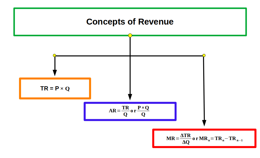
Revenue The income earned by a producer by selling output in the market is called revenue.
Revenues are classified into:- 1. Total revenue (TR)
- 2. Average revenue (AR)
- 3. Marginal revenue (MR)
1. Total revenue (TR) The amount of money a production unit gets by selling all its output is called total revenue. Under perfect competition TR is calculated by multiplying market price (p) with the quantity of goods (q), i.e.,
$$ \mathbf{TR\,=\, p\,×\,q} $$ Price in a perfectly competitive market is constant. In the below Table 4.1 the price of output and the different quantities of the output are given.| Table 4.1 | ||
|---|---|---|
| Price (P) | Quantity (Q) | Total Revenue = P×Q |
| 10 | 0 | 0 |
| 10 | 1 | 10 |
| 10 | 2 | 20 |
| 10 | 3 | 30 |
| 10 | 4 | 40 |
| 10 | 5 | 50 |
| 10 | 6 | 60 |
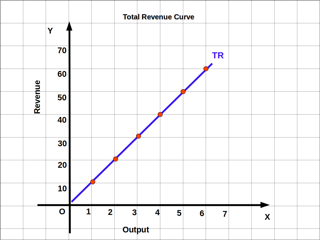 Three important points are to be noted from this graph.
- 1). When output is zero, TR will also be zero. So TR curve starts from origin.
- 2). As output increases TR also increases. Moreover TR curve is an upward rising straight line with positive slope.
- 3). The slope of the TR curve will be constant, i.e., the slope of TR curve will be equal to the market price.
Price Line The line that shows the relation between output and price is known as price line. In a perfectly competitive market, the output of a firm does not depend on price. This means, any number of output can be sold at same price. So the price line under perfect competition is always parallel to x-axis. In Table 4.1 the price of the product is ₹10. As the unit of output increases no change occurs in the price.
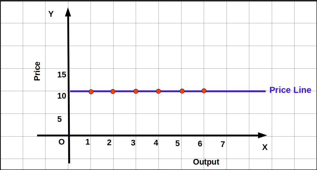 Price is marked along the y-axis and the output is marked along the x-axis. Price-output combinations are used to draw the above given Graph and we get a horizontal line. This is known as price line.
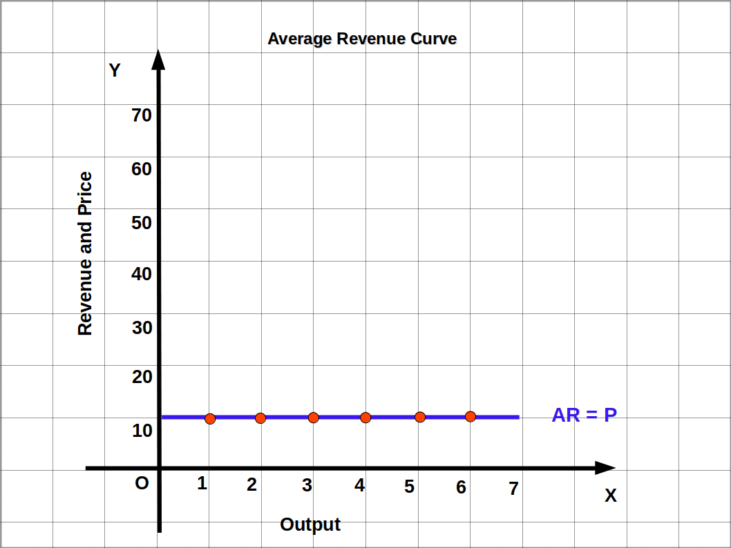
2. Average revenue (AR) Total revenue per unit of output is called average revenue. AR is calculated by dividing TR by quantity of output sold.
$$ \mathbf{AR\,=\,\frac{TR}{Q}=\frac{P×Q}{q}=P} $$ AR is equal to price. Therefore, price line and AR curve are one and the same. That is why AR curve and demand curve of a firm under perfect competition are also one and the same.| Table 4.2 | |||
|---|---|---|---|
| Price (P) | Quantity (Q) | TR = P×Q | \(\mathbf{AR=\frac{TR}{Q}}\) |
| 10 | 0 | 0 | 0 |
| 10 | 1 | 10 | 10÷1=10 |
| 10 | 2 | 20 | 20÷2=10 |
| 10 | 3 | 30 | 30÷3=10 |
| 10 | 4 | 40 | 40÷4=10 |
| 10 | 5 | 50 | 50÷5=10 |
| 10 | 6 | 60 | 60÷6=10 |
3. Marginal revenue (MR) MR is the addition to the total revenue when an additional unit of output is sold. It can also be defined as change in TR (ΔTR) divided by change in output sold (ΔQ).
Algebraically, $$ \mathbf{MR\,=\,\frac{ΔTR}{ΔQ}} $$ $$ \mathbf{or} $$ $$ \mathbf{MR_{n}\,=\,TR_{n}-TR_{n-1}} $$ (where n is the number of units of output sold) It is to be noted that the sum of MR of all the units of a commodity sold is equal to TR, Symbolically: $$ \mathbf{TR\,=\,Σ\,MR} $$ Under perfect competition, at any level of output MR and market price are equal. So the shape of MR curve will be a line parallel to x-axis. Look at Table 4.3. When quantity increases from 0 to 1 TR increases from 0 to = ₹ 10. Then, MR1 = TR1 – TR0 = 10 – 0 = ₹ 10. When 2 units are sold, TR is ₹ 20. Then, MR2 = TR2 – TR1 = 20 – 10 = ₹ 10.| Table 4.3 | ||
|---|---|---|
| Product (Q) | TR | \(\mathbf{MR = \frac{ΔTR}{ΔQ}}\) |
| 0 | 0 | – |
| 1 | 10 | 10 ÷ 1 = 10 |
| 2 | 20 | 10 ÷ 1 = 10 |
| 3 | 30 | 10 ÷ 1 = 10 |
| 4 | 40 | 10 ÷ 1 = 10 |
| 5 | 50 | 10 ÷ 1 = 10 |
| 6 | 60 | 10 ÷ 1 = 10 |
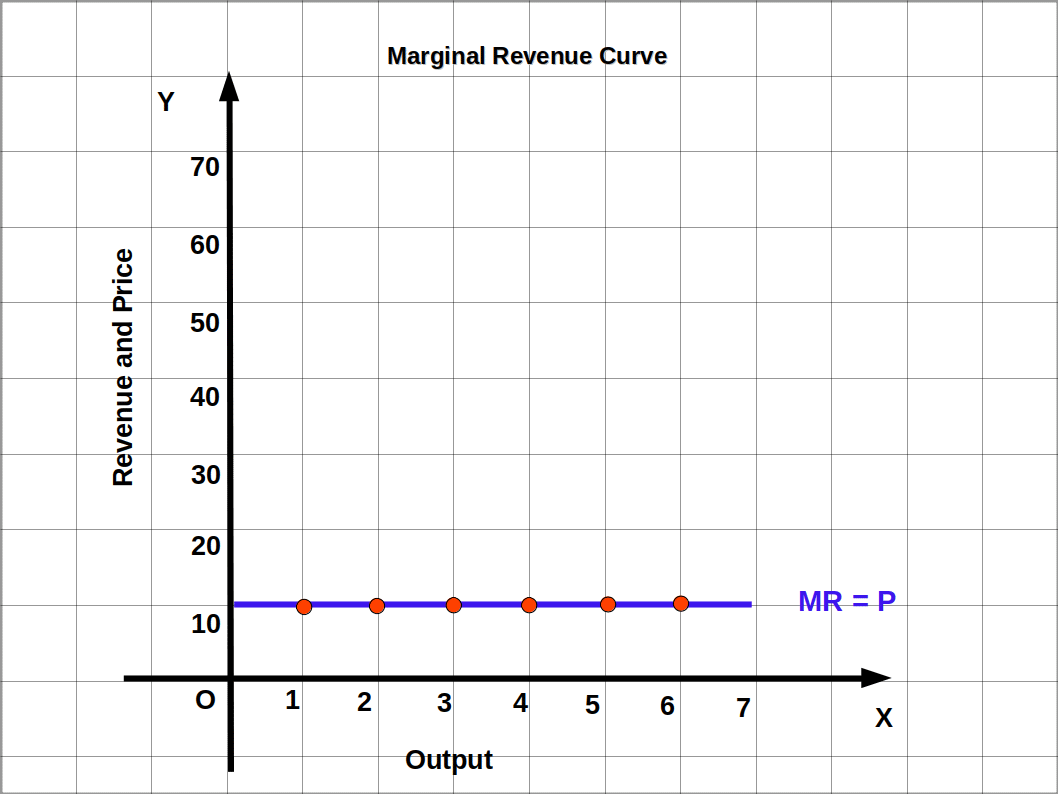 Under perfect competition,
\(\mathbf{P=AR=MR}\)
| Table 4.4 | ||
|---|---|---|
| Price | Product | |
| 5 | 0 | |
| 5 | 1 | |
| 5 | 2 | |
| 5 | 3 | |
| 5 | 4 | |
| 5 | 5 | |
| Table 4.5 | ||||
|---|---|---|---|---|
| P | Q | TR=P×Q | \(\mathbf{AR=\frac{TR}{Q}}\) | \(\mathbf{MR=\frac{ΔTR}{ΔQ}}\) |
| 5 | 0 | 0 | – | – |
| 5 | 1 | 5 | 5 | 5 |
| 5 | 2 | 10 | 5 | 5 |
| 5 | 3 | 15 | 5 | 5 |
| 5 | 4 | 20 | 5 | 5 |
| 5 | 5 | 25 | 5 | 5 |
Profit Maximisation Every producer produces goods and services and sells them in the market. The main objective of every production unit is to maximise its profit. Equilibrium is reached at the point of maximum profit. It is the state in which the producer has no tendency to increase or decrease the quantity of output sold. Profit x is the difference between the Total Revenue (TR) and Total Cost (TC). i.e.,
Algebraically,\(\mathbf{π\,=\,TR\,-\,TC}\)
A firm reaches equilibrium when the difference between TR and TC is maximum. The difference between TR and TC will be maximum when the following three conditions are satisfied.
- (1) Market Price (P) should be equal to the marginal cost (MC)
- (2) MC should be non-decreasing. In other words, the MC curve should cut the MR curve from below.
- (3)
- (a) Price should be greater than or equal to AVC in the short run.
(b) Price should be greater than or equal to Long-run Average Cost.
\(\mathbf{P\,≥\,AVC}\)
\(\mathbf{P\,≥\,LRAC}\)
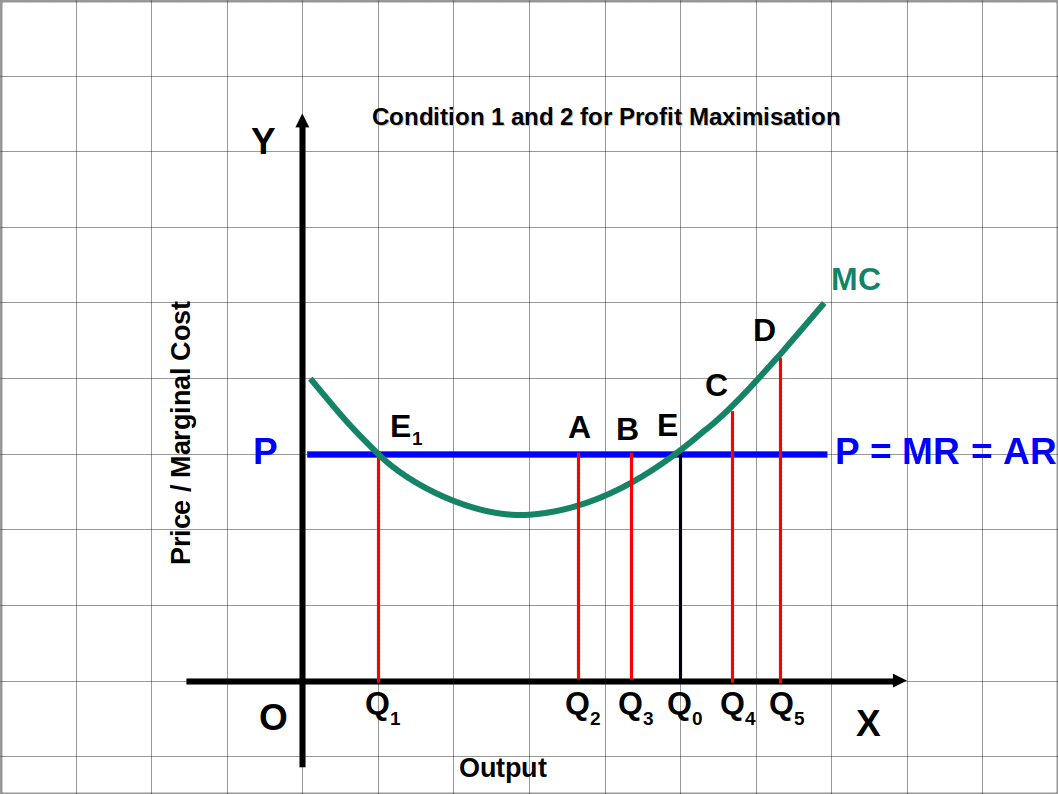 In the above Diagram output is marked on the X axis and price/MC is on the y axis. MC is the marginal cost curve and P = AR = MR is the price line. When output increases, MC decreases initially and then increases. (P > MC). At the output level from Q1 to Q0 the market price is higher than MC. At point E the firms profit reaches its maximum at Q0 level of output. So the firm would not attain maximum profit when price is greater than MC. In this case a firm can maximize profit by increasing the quantity of output.
Case 2: Price less than MC is ruled out
In the case of price less than MC (before Q1 and after Q0) the firm incurs losses.
Condition 2: MC curve should cut MR curve from below.
(MC should be non-decreasing at equilibrium.)
The second condition for equilibrium requires that the MC curve should cut the MR curve from below. This means the marginal cost (MC) should be non-decreasing at equilibrium. In the diagram MC and MR are equal at two points E and E1. But there can be only one equilibrium point. Point E1 cannot be the equilibrium point even though MC and MR are equal. This is because
MC curve cuts MR curve from above; MC curve is decreasing. At point E, MR and MC are equal and MC is non-decreasing (rising). Here, MC curve cuts MR curve from below. At Q0 the firm reaches equilibrium and attains Profit maximising level of output.
Condition 3: Condition 3 has two parts, one for the short run and another for the long run.
Case 1: Price should be greater than or equal to AVC in the short run.
In the short run, a profit maximising firm will not produce at an output level where market price is lower than AVC.
In the above Diagram output is marked on the X axis and price/MC is on the y axis. MC is the marginal cost curve and P = AR = MR is the price line. When output increases, MC decreases initially and then increases. (P > MC). At the output level from Q1 to Q0 the market price is higher than MC. At point E the firms profit reaches its maximum at Q0 level of output. So the firm would not attain maximum profit when price is greater than MC. In this case a firm can maximize profit by increasing the quantity of output.
Case 2: Price less than MC is ruled out
In the case of price less than MC (before Q1 and after Q0) the firm incurs losses.
Condition 2: MC curve should cut MR curve from below.
(MC should be non-decreasing at equilibrium.)
The second condition for equilibrium requires that the MC curve should cut the MR curve from below. This means the marginal cost (MC) should be non-decreasing at equilibrium. In the diagram MC and MR are equal at two points E and E1. But there can be only one equilibrium point. Point E1 cannot be the equilibrium point even though MC and MR are equal. This is because
MC curve cuts MR curve from above; MC curve is decreasing. At point E, MR and MC are equal and MC is non-decreasing (rising). Here, MC curve cuts MR curve from below. At Q0 the firm reaches equilibrium and attains Profit maximising level of output.
Condition 3: Condition 3 has two parts, one for the short run and another for the long run.
Case 1: Price should be greater than or equal to AVC in the short run.
In the short run, a profit maximising firm will not produce at an output level where market price is lower than AVC.
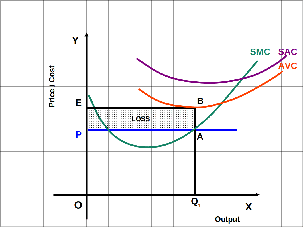 It is clear from the above diagram that at OP price level the firm produces OQ1 level of output. It is lower than AVC.
At this point TR = Price × Quantity
= OP × OQ1, (The area OPAQ1)
Similarly, TVC of the Firm at Q1 level of output = AVC × Quantity
= OE × OQ1, (The area OEBQ1)
Here we can see that the expenditure is higher than revenue (OEBQ1 > OPAQ1)
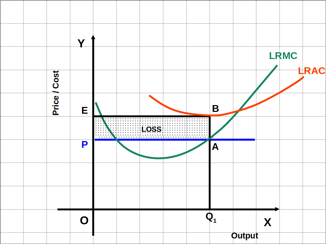
Hence the firm’s loss at zero output is equal to TFC. Therefore, the firm produces nothing when the price is less than AVC, in the short run. So Q1 is not a profit maximising output level. Therefore condition 3 (case 1) is that, in the short run price should be greater than or equal to AVC.
It is clear from the above diagram that at OP price level the firm produces OQ1 level of output. It is lower than AVC.
At this point TR = Price × Quantity
= OP × OQ1, (The area OPAQ1)
Similarly, TVC of the Firm at Q1 level of output = AVC × Quantity
= OE × OQ1, (The area OEBQ1)
Here we can see that the expenditure is higher than revenue (OEBQ1 > OPAQ1)
Hence the firm’s loss at zero output is equal to TFC. Therefore, the firm produces nothing when the price is less than AVC, in the short run. So Q1 is not a profit maximising output level. Therefore condition 3 (case 1) is that, in the short run price should be greater than or equal to AVC.

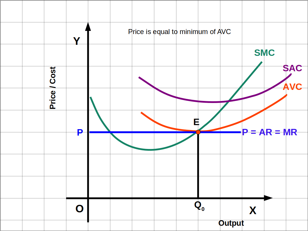
In short run the price of the product should be equal to, or more than, the minimum AVC. In the below diagram at Q0 price at point E is equal to the minimum AVC. If no production takes place in short run, the loss suffered by the producer is equal to TFC. If price is below AVC loss would be more than TFC. Stopping production is better than producing at a price below AVC. But if price is at minimum AVC loss would be only TFC. Producing at this level is better. If price is a above the AVC, minimum point loss can be reduced by increasing production. Therefore in short run product price must be either minimum AVC or more than that.
 In short run, if the price of the product is more than the minimum of AVC, the firm will get profit. In the below diagram at Q0 price at point A is above the minimum of AVC. Firm will get profit equal to the area EPAB as shown in the diagram. In such a situation, revenue is more than cost (OPAQ0 > OEBQ0). So the firm can produce more output, till the revenue equals cost. Therefore in short run, if price is more than minimum of AVC firm will get profit.

 In the Diagram, firm’s TR at Q1 level of output is the area OPAQ1 while the firm’s TC is the area OEBQ1. Here the firm incurs loss at Q1 level of output (OEBQ1 > OPAQ1). In such a situation the firm will have to shut down production. So Q1 is not a profit maximising output level. Therefore, condition 3 (case 2) is that, in the long run, price should be greater than or equal to average cost (AC).

In the long run, price should be equal to, or more than , the minimum AC. If price is equal to LRAC the firm will be at no profit, no loss level. In this condition the firm will have normal profit.
π = TR – TC = OPEQ0 – OPEQ0 = 0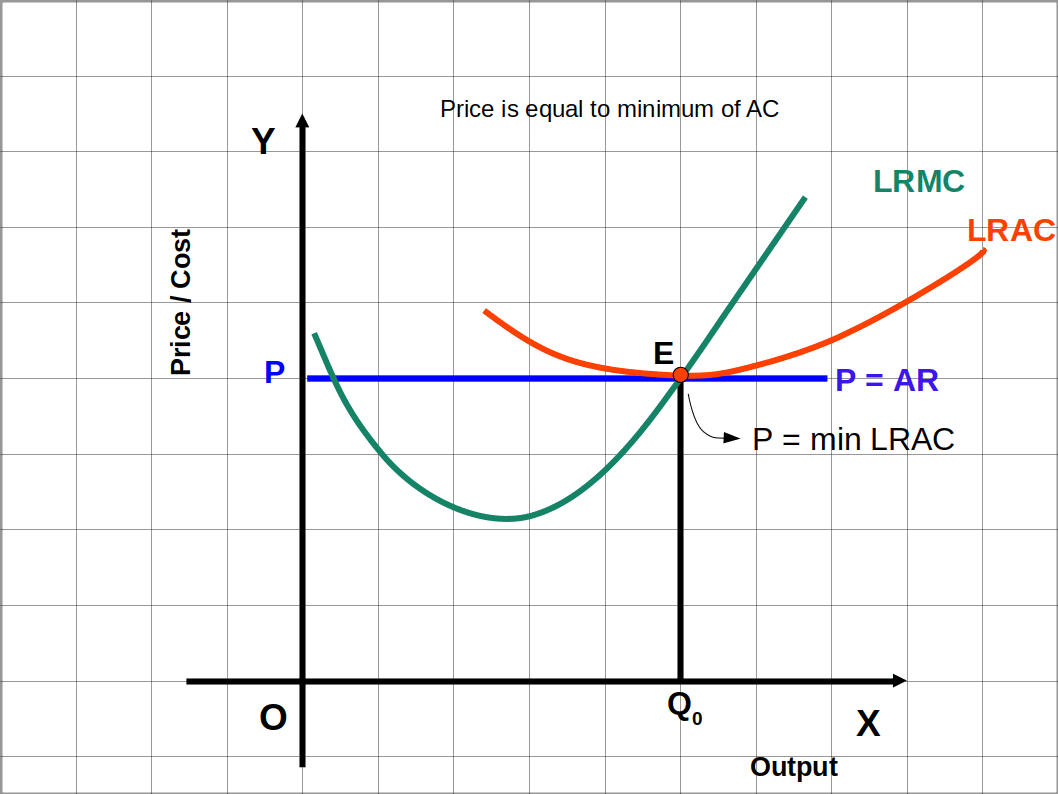
Supply The quantity of a commodity that a firm offers to sell in the market at different prices in a given period of time is called supply.
Supply Curve of a Firm The graph that represents the different quantities of a commodity that a firm offers to sell in the market at different prices in a given period of time is called the supply curve of the firm. We have short run and long run supply curve.
Short-run Supply Curve of a Firm Short-run supply curve of a firm is defined as the rising portion of the SMC curve from and above minimum AVC. In Diagram 4.5, the bold rising portion of SMC curve is the short-run supply curve.
We shall discuss how the short-run supply curve is formed from the SMC curve of a firm that tries to maximise profit. Derivation of the short-run supply curve can be explained in two circumstances. Case 1: Price is greater than or equal to the minimum AVC. Case 2: Price is less than the minimum AVC. Case 1: Price is greater than or equal to the minimum AVC When price is minimum AVC the output of the firm will be positive. If price is more than the minimum AVC, the supply will increase along with the increase in price. In below Diagram, when price is P1, price and SMC are equal at equilibrium point E1 and the firm produces q1 quantity of output. At point E1 all the three conditions of short-run equilibrium under perfect competition are fulfilled.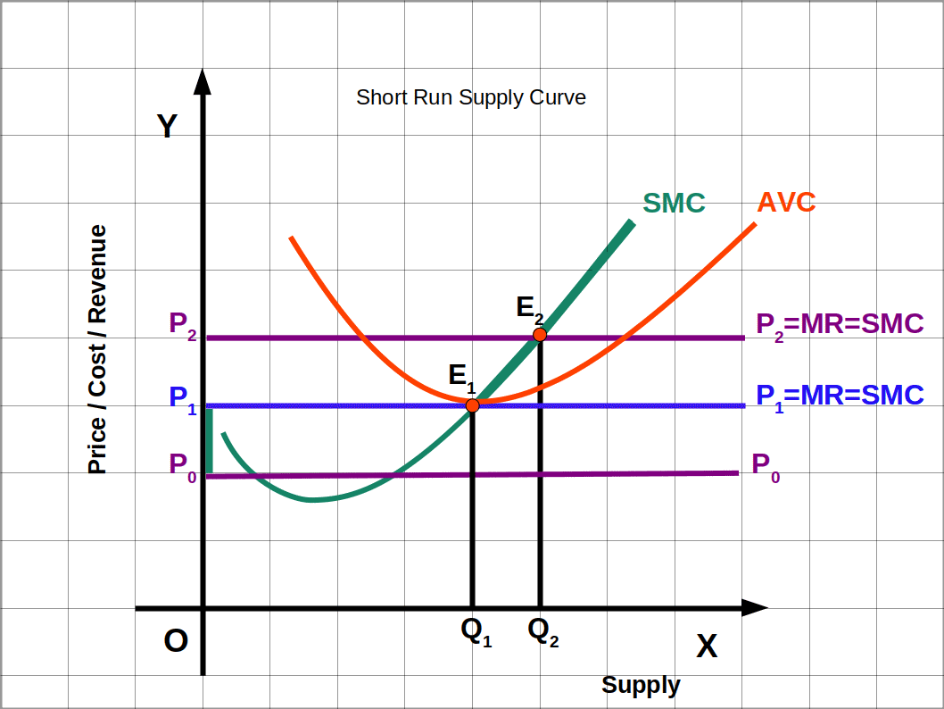 If price is more than the minimum AVC the output increases. In the diagram when price increases from P1 to P2, the price line and the SMC curve intersect at the equilibrium point E2. At the point E2, the output that attains maximum profit increases from q1 to q2. That means when price increases supply also increases. The bold portion of SMC curve is short run supply curve.
Case 2: Price is less than the minimum AVC.
If price is less than the minimum AVC, supply would be zero. In the above Diagram, if price is P0 the firm will not produce. P0 is below shutdown point. In this situation the third condition of equilibrium is not fulfilled. Therefore, at any price below the minimum AVC, supply would be zero.
The derivation of short run supply curve can be summarised as follows:
If price is more than the minimum AVC the output increases. In the diagram when price increases from P1 to P2, the price line and the SMC curve intersect at the equilibrium point E2. At the point E2, the output that attains maximum profit increases from q1 to q2. That means when price increases supply also increases. The bold portion of SMC curve is short run supply curve.
Case 2: Price is less than the minimum AVC.
If price is less than the minimum AVC, supply would be zero. In the above Diagram, if price is P0 the firm will not produce. P0 is below shutdown point. In this situation the third condition of equilibrium is not fulfilled. Therefore, at any price below the minimum AVC, supply would be zero.
The derivation of short run supply curve can be summarised as follows:

- If price is less than minimum AVC, supply would be zero
- If it is the minimum AVC, supply would be positive
- If it is more than the minimum AVC, supply will increase
Long-run supply curve of a firm The long-run supply curve of a firm can be defined as the rising portion of the LRMC curve from and above the minimum LRAC together with zero output. In the Diagram, the bold rising portion of the LRMC curve is the long run supply curve.
Derivation of long-run supply curve can be explained in two circumstances: Case 1: Price greater than or equal to the minimum LRAC. Case 2: Price less than the minimum LRAC. Case 1: Price greater than or equal to the minimum LRAC. When price is equal to minimum LRAC, output is positive. If price is more than minimum LRAC, supply will increase as the price increases. In the below Diagram when price is P1, price and LRMC become equal. The firm produces and supplies q1 amount of output, at equilibrium point E1. At q1 output all the three conditions of long-run equilibrium are fulfilled. Price P1 is the minimum LRAC.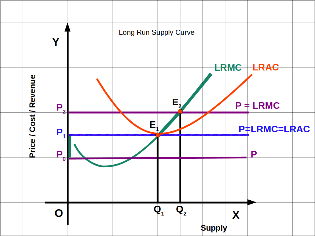 If price is more than LRAC, the quantity of output increases. In the diagram, when price increases from P1 to P2 the price line and SMC curve intersect at the equilibrium point E2. At this point, the level of profit maximising output increases from q1 to q2 . When price increases equilibrium supply also increases.
Case 2: Price less than the minimum LRAC.
When price falls below minimum LRAC, output would be zero. In the above Diagram, if price is P0 the firm will not produce. Price P1 is below E1. In this case, the third condition of equilibrium is not satisfied. So, at any price below the minimum LRAC, supply would be zero.
The derivation of long-run supply curve can be summarised as follows:
If price is more than LRAC, the quantity of output increases. In the diagram, when price increases from P1 to P2 the price line and SMC curve intersect at the equilibrium point E2. At this point, the level of profit maximising output increases from q1 to q2 . When price increases equilibrium supply also increases.
Case 2: Price less than the minimum LRAC.
When price falls below minimum LRAC, output would be zero. In the above Diagram, if price is P0 the firm will not produce. Price P1 is below E1. In this case, the third condition of equilibrium is not satisfied. So, at any price below the minimum LRAC, supply would be zero.
The derivation of long-run supply curve can be summarised as follows:
- If price is less than minimum LRAC, supply would be zero.
- If price is equal to minimum LRAC, supply would be positive.
- If price is more than minimum LRAC, supply will increase.
Shut down point (Short run) The situation in which a firm stops production and leaves the market is called shut down point. In the short run, the firm should get a minimum price for the product to meet the AVC. If the firm cannot meet the AVC, it has to stop production. and shut down the firm. If the firm has to continue production it should get a price equal to minimum AVC where SMC cuts the AVC. So the minimum point of AVC is called short run shut down point.
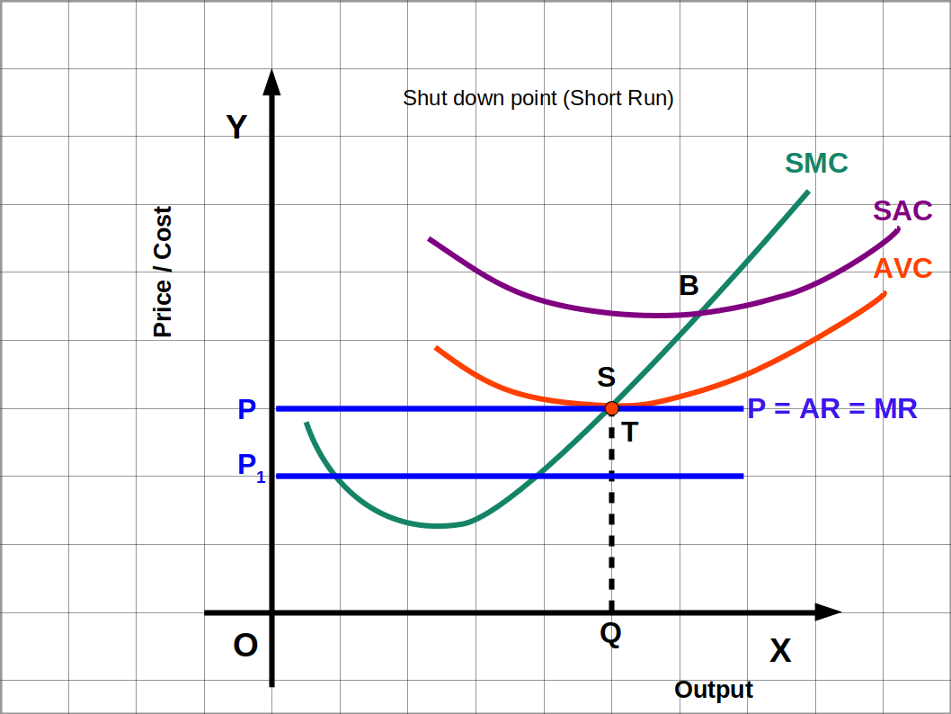 In the above given Diagram, at point S price OP and AVC are equal. This price is equal to the minimum AVC. At price OP the firm produces OQ output. If the price goes down to OP1 it will stop production and shut down the unit. So point S is the shut down point in the short run.
Shut down point (Long run) In the long run, minimum LRAC is the shut down point. A firm that tries to maximise profit in the long run, will stop production if the price is less than LRAC.
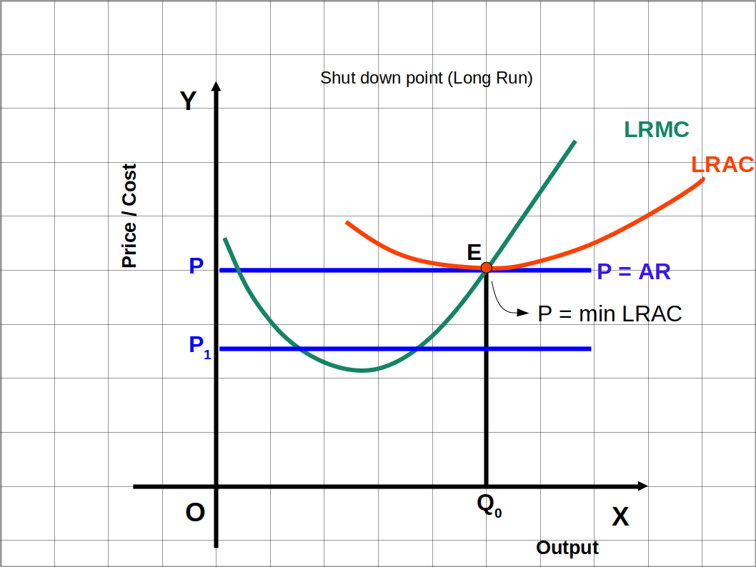 In the above Diagram, at point E, price and minimum LRAC are equal. Then price is OP and output is OQ0. If price goes down from OP to OP1 cost will be greater than revenue. So the firm will stop production and shut down the unit. So point E is the shut down point in the long run.

Shut Down Point
- P = minimum AVC (Short run).
- P = minimum LRAC (Long run).
Types of Costs
Explicit Cost is the cost incurred by the producer for purchasing or hiring inputs. For example wages, interest, rent, cost of raw material, etc..
Implicit Cost is the costs of self owned and self supplied factors in one’s own business. In economics, the sum of implicit costs and explicit costs constitutes the total cost of production of a commodity. Opportunity Cost is the incomes from the next best alternative that is foregone when the entrepreneur makes certain choices. For example, the entrepreneur could have earned a salary had he worked for others instead of spending time on his own business. These costs calculate the missed opportunity and calculate income that we can earn by following some other policy. Sunk Cost is the costs that will not be recovered by the business. They cannot be gotten back regardless of what happens. They are excluded from future business decisions. If you have invested money in a business that has gone bankrupt, it is a sunk cost already (even though you may recuperate some of the revenue through the court system) Operating Cost is the sometimes referred to as operating expenses. These can be either fixed or variable. Operating costs are costs that are associated with daily business activity but are distinct from indirect costs. Rent and utilities are typical examples of operating costs. They are essential for business operations but are not involved in the manufacturing process directly or indirectly.Normal Profit The normal profit is the level of profit which is just enough to cover the explicit and opportunity Costs of the firm.
The minimum profit that a firm earns in order to stay in the industry is normal profit. This is the minimum profit for a firm to continue production in the industry. In the short run, even though the firm makes a profit which is less than normal profit, production may continue. But in the long run if it gets profit less than the normal profit, it will stop production. In the long run, all firms: will earn only normal profit.Super Normal Profit (Abnormal Profit) The profit that a firm earns over and above normal profit is called super normal profit. In the short run, some firms may get super normal profits, while other firms may incur losses. But in the long run, all firms earn normal profit.
Break-even Point The situation in which the total revenue of a firm equals total cost (TR = TC) is called break-even point or no profit no loss point. In other words, break-even point is the point on the supply curve at which a firm earns normal profit.
In the short run, the minimum point of SAC curve, and in the long run, the minimum point of the LRAC curve are called break-even point or no profit-no loss point.Determinants of a firm’s supply curve Supply curve of a firm is a part of MC curve. Therefore, any factor that affects the MC curve will definitely be the determinant of the supply curve. Price of commodity, technology of production, input costs and unit tax are the important factors that affect supply curve. We shall now discuss how these factors influence the supply curve.
1. Price of the commodity The most important factor that determines supply of a commodity is its price. There is a direct or positive relation between price and quantity supplied. When price of commodity rises its quantity supplied also rises and vice versa.
2. Technology of production Suppose a firm uses capital and labour as factors of production to produce a certain good. With improved technology or innovation, a firm can produce more units of output with the same level of input or same level of output with less amount of input. When improved technology (organisational innovation) is used, MC decreases and the supply curve shifts to the right or downwards. On the other hand, when outdated technology is used MC increases and the supply curve shifts to the left or upwards. At any given market price, the firm can supply more units of output.
3. Input prices The supply of a firm is influenced by the prices of inputs. If input prices go down, MC will decrease. As a result the supply curve will shift to the right. Similarly, if input prices go up, MC will increase and the supply curve will shift to the left. At any given market price, the firm can supply lower units of output.
4. Unit tax A unit tax is a tax that the government imposes per unit sale of output. When unit tax is increased MC increases and the supply curve shifts to the left. Similarly, when unit tax is reduced, the supply curve shifts to the right. This can be better explained with the help of below given Diagram.
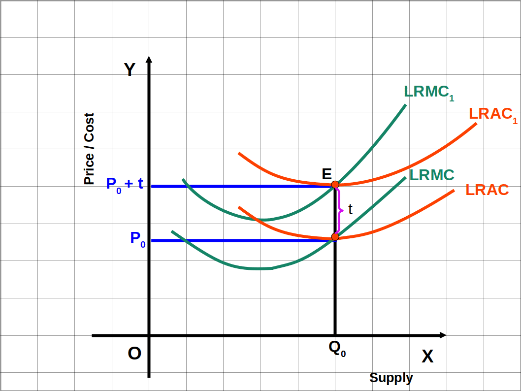 In the above Diagram, at P0 price the supply is Q0. The government increases tax by ₹ t per unit. So LRAC and LRMC increase by ₹ t. Hence LRAC and LRMC curves move upwards
and become LRAC1 and LRMC1. So the new price is the old price P0 and tax ₹ t. ie., P0 + t.
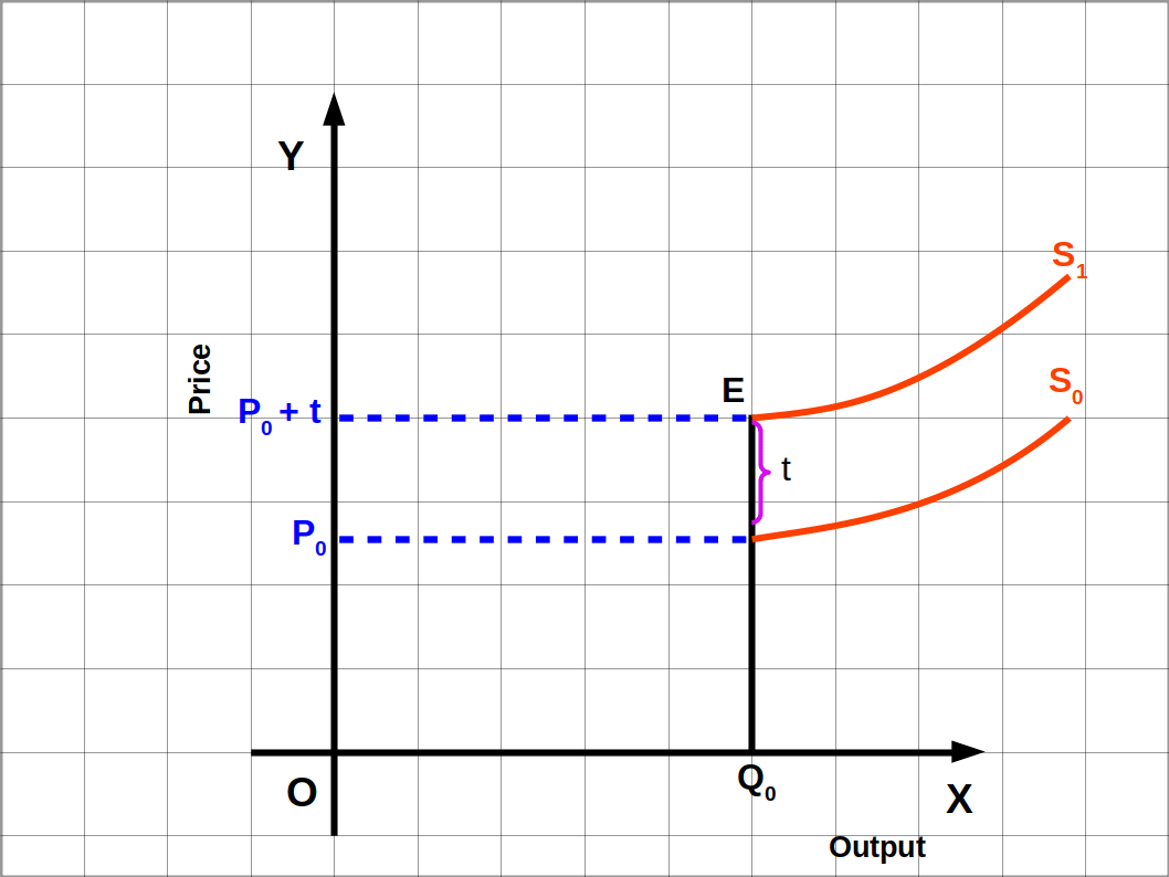
Long run supply curve starts from the minimum of LRAC curve and goes upwards. In the below Diagram, S0 and S1 respectively are the supply curves before unit tax and after unit tax. That means the supply curve S0 becomes S1 after tax and shifts towards the left.
In the above Diagram, at P0 price the supply is Q0. The government increases tax by ₹ t per unit. So LRAC and LRMC increase by ₹ t. Hence LRAC and LRMC curves move upwards
and become LRAC1 and LRMC1. So the new price is the old price P0 and tax ₹ t. ie., P0 + t.
Long run supply curve starts from the minimum of LRAC curve and goes upwards. In the below Diagram, S0 and S1 respectively are the supply curves before unit tax and after unit tax. That means the supply curve S0 becomes S1 after tax and shifts towards the left.
Supply Function The functional relationship between supply of a commodity and the determinants of supply is called supply function, i.e., the relationship between supply (S) and its determinants such as price of the commodity (P), Technology of production (T), Input prices or cost of factors of production (F) and unit tax (t)
Algebraically,\(\mathbf{S=f(P,T,F,t)}\)
The price, p is the most important factor among the determinants of supply. Therefore, the supply of a commodity can be written as the function of price.
\(\mathbf{S=f(P)}\)
Law of Supply The positive relationship between price and quantity supplied is known as law of supply. Law of supply states that, “Other things remaining unchanged, when the price of a commodity rises its quantity supplied also rises and vice versa”. It is based on the assumption that technology of production, input prices and unit tax are constant.
When the price of paddy rises from ₹ 15 to ₹ 20 per kg, a farmer was ready to increase its supply from 1,000 kg to 2,000 kg. In this situation price of paddy rises and the quantity supplied of paddy also rises. On the other hand, if price of paddy decreases from ₹ 15 to ₹ 10 the farmer is ready to supply only 500 kg. Here the price of paddy falls, quantity supplied of paddy also falls. Thus the positive relation between price and supply is called the law of supply.Supply function equation Supply function equation states the relation between price and supply. If S is supply and P is price, the law of supply can be stated algebraically as
 In this supply function equation ‘a’ is a constant value. If price is less than ‘a’ supply would be 0. If price is greater than or equal to ‘a’ supply function would be S = P – a.
The supply function equation of a firm is given below:
In this supply function equation ‘a’ is a constant value. If price is less than ‘a’ supply would be 0. If price is greater than or equal to ‘a’ supply function would be S = P – a.
The supply function equation of a firm is given below:
 The first part of this equation shows that if price is less than ₹ 10, supply would be 0. The second part of the supply function equation shows that when price is ₹ 10 or above, supply would be 0. For example, if price is ₹ 9. S = 9 – 10 = -1. Since supply is negative it is considered as 0. The supply of commodity is given in Table 4.6 when price varies from ₹ 10 to ₹15.
When price increases as 10, 11, 12, 13, 14, 15 the supply increases as 0, 1, 2, 3, 4, 5 respectively. Therefore, the equation S = P – 10 shows the positive relation between price and supply.
The first part of this equation shows that if price is less than ₹ 10, supply would be 0. The second part of the supply function equation shows that when price is ₹ 10 or above, supply would be 0. For example, if price is ₹ 9. S = 9 – 10 = -1. Since supply is negative it is considered as 0. The supply of commodity is given in Table 4.6 when price varies from ₹ 10 to ₹15.
When price increases as 10, 11, 12, 13, 14, 15 the supply increases as 0, 1, 2, 3, 4, 5 respectively. Therefore, the equation S = P – 10 shows the positive relation between price and supply.
| Table 4.6 Individual Supply Schedule | ||
|---|---|---|
| Price | Supply = P – 10 | |
| 9 | 0 | |
| 10 | 10 – 10 = 0 | |
| 11 | 11 – 10 = 1 | |
| 12 | 12 – 10 = 2 | |
| 13 | 13 – 10 = 3 | |
| 14 | 14 – 10 = 4 | |
| 15 | 15 – 10 = 5 | |
Individual Supply Schedule Individual Supply Schedule is a table showing the different quantities of a good or service at different prices that a producer is willing to sell in a market. Table 4.6 is an individual supply schedule.
The supply function of a firm is given below:
| Table 4.7 Individual Supply Schedule | ||
|---|---|---|
| Price | Supply = 2P – 40 | |
| 20 | 2 × 20 – 40 = 40 – 40 = 0 | |
| 21 | 2 × 21 – 40 = 42 – 40 = 2 | |
| 22 | 2 × 22 – 40 = 44 – 40 = 4 | |
| 23 | 2 × 23 – 40 = 46 – 40 = 6 | |
| 24 | 2 × 24 – 40 = 48 – 40 = 8 | |
| 25 | 2 × 25 – 40 = 50 – 40 = 10 | |
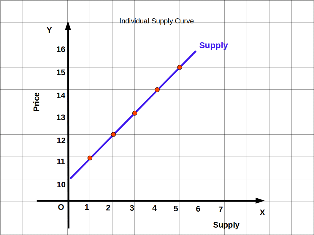
Individual Supply Curve The graphical representation of an individual supply schedule is called individual supply curve. It is a graph that shows the relation between the price of a commodity and its supply.
The individual supply curve given below is the graph based on Table 4.8. In this graph price is marked on the y-axis and supply on the x-axis. Line SS is the supply curve. This shows the Positive relation between price and supply. When price is 9 and 10, supply is 0. When price increases from 10 to 11, 12, 13, 14 and 15 supply also increases as 1, 2, 3, 4 and 5 respectively.| Table 4.8 Individual Supply Schedule | ||
|---|---|---|
| Price | Supply | |
| 9 | 0 | |
| 10 | 0 | |
| 11 | 1 | |
| 12 | 2 | |
| 13 | 3 | |
| 14 | 4 | |
| 15 | 5 | |
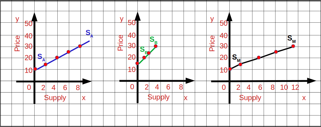
Market Supply Market supply is the sum of quantities supplied by all the producers in the market at a given price. This is the sum total of all the quantities of a commodity sold by all the firms in the market at various prices.
There are three producers of paddy – A, B and C. A supplies 100 kg paddy at the rate of ₹ 15/kg, B 50 kg and C 200 kg. So at ₹ 15 market supply is Sm = 100 + 50 + 200 = 350 kg.Market Supply Schedule Horizontal summation of all individual supply schedules is the market supply schedule. The market supply schedule is obtained by adding all the quantities supplied by all the producers of the same product at different prices in the market.
How a market supply schedule has been Prepared from the individual supply schedules of two different producers A, and B is shown below.| Table 4.9 Individual Supply Schedule and Market Supply Schedule | |||||
|---|---|---|---|---|---|
| Individual A | Individual B | Market Supply (Supply A + Supply B) |
|||
| Price | Supply | Price | Supply | Price | Supply |
| 10 | 0 | 10 | 0 | 10 | 0 |
| 15 | 2 | 15 | 0 | 15 | 2 |
| 20 | 4 | 20 | 1 | 20 | 5 |
| 25 | 6 | 25 | 2 | 25 | 8 |
| 30 | 8 | 30 | 3 | 30 | 11 |
Market Supply Curve The graph of the market supply schedule is called market supply curve. Market supply curve is obtained by horizontal summation of all individual supply curves.
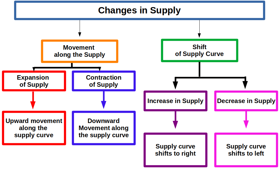
Changes in Supply There are two types of changes in supply. They are: (I) movement along the supply curve (II) shift of supply curve.
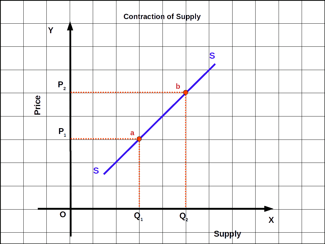
I. Movement along the Supply Curve Change in the supply due to change in price is called movement along the supply curve. They are:
- (a) Expansion of supply
- (b) Contraction of supply
(a) Expansion of supply The upward movement along the supply curve due to a rise in price is called expansion of supply, i.e., rise in quantity supplied due to a rise in price is called expansion of supply. In below Diagram, when price rises from P1 to P2, supply rises from Q1 to Q2 along the supply curve SS. The upward movement from point a to b is called expansion of supply.

(b) Contraction of supply The downward movement along the supply curve due to a fall in price is called contraction of supply. i.e., a fall in quantity supplied due to a fall in price is called contraction of supply. In below Diagram, when price falls from P2 to P1, supply falls from Q2 to Q1. The downward movement along the supply curve SS from point b to a is called contraction of supply.
II. Shift of Supply Curve The change in supply due to change in non-price factors like price of input, technology, unit tax, prices of other commodities, climate, etc., is called shift of supply curve. This can be two types:
- (a) Increase in supply
- (b) Decrease in supply
(a) Increase in supply The rightward shift of supply curve due to decrease in input price, tax reduction, favourable changes in technology, etc., is called increase in supply. This can be defined in two ways:
- (a) More quantity is supplied at a given price.
- (b) Same quantity is supplied at lower price.
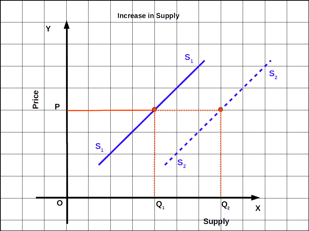 Supply curve S1 shifts rightward as S2 due to increase in supply. At price OP, OQ2 quantity is supplied. That means more quantity is supplied at a given price. This is called increase in supply.
(b) Decrease in supply The leftward shift of supply curve due to increase in input.price, increase in unit tax, adverse changes in technology, ete., is called decrease in supply. Decrease in supply can be defined in two different ways:
- (a) Less quantity is supplied at the given price.
- (b) Same quantity is supplied at higher price.
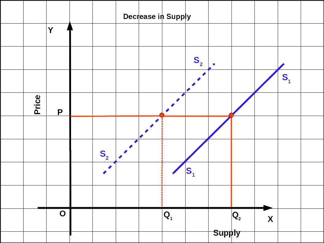 As a result of decrease in supply the supply curve S, shifts to the left as S2. Now at the same price OP the quantity supplied is OQ1, i.e., at the same price, less quantity is supplied. This is called decrease in supply. Increase and decrease in supply is caused by changes in non-price factors.
Price Elasticity of Supply Price elasticity of supply is defined as the degree of responsiveness of quantity supplied of a commodity with respect to change in its price. The price elasticity of supply can be calculated by dividing the percentage change in supply by the percentage change in price.
Degrees of Price Elasticity of Supply On the basis of change in quantity supplied, elasticity can be classified into five types. They are:
- (1) High elasticity of supply
- (2) Inelastic supply or less elasticity of supply
- (3) Unitary elastic supply
- (4) Perfectly elastic supply
- (5) Perfectly inelastic supply
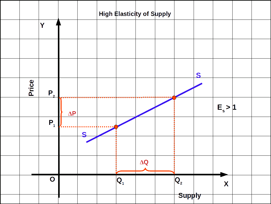
(1) High elasticity of supply ( es > 1 ) When percentage change in supply is more than the percentage change in price it is called high elasticity of supply. In such cases, the slope of the supply curve will be less, as seen in below Diagram. Value of elasticity will be more than one.
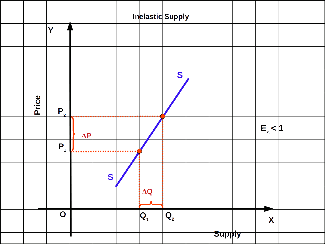
(2) Inelastic supply or less elasticity of supply ( es < 1 ) If percentage change in supply is less than the percentage change in price it is called inelastic supply. In this case, the slope of the supply curve will be high, as seen in the below Diagram. Value of elasticity will be less than one.
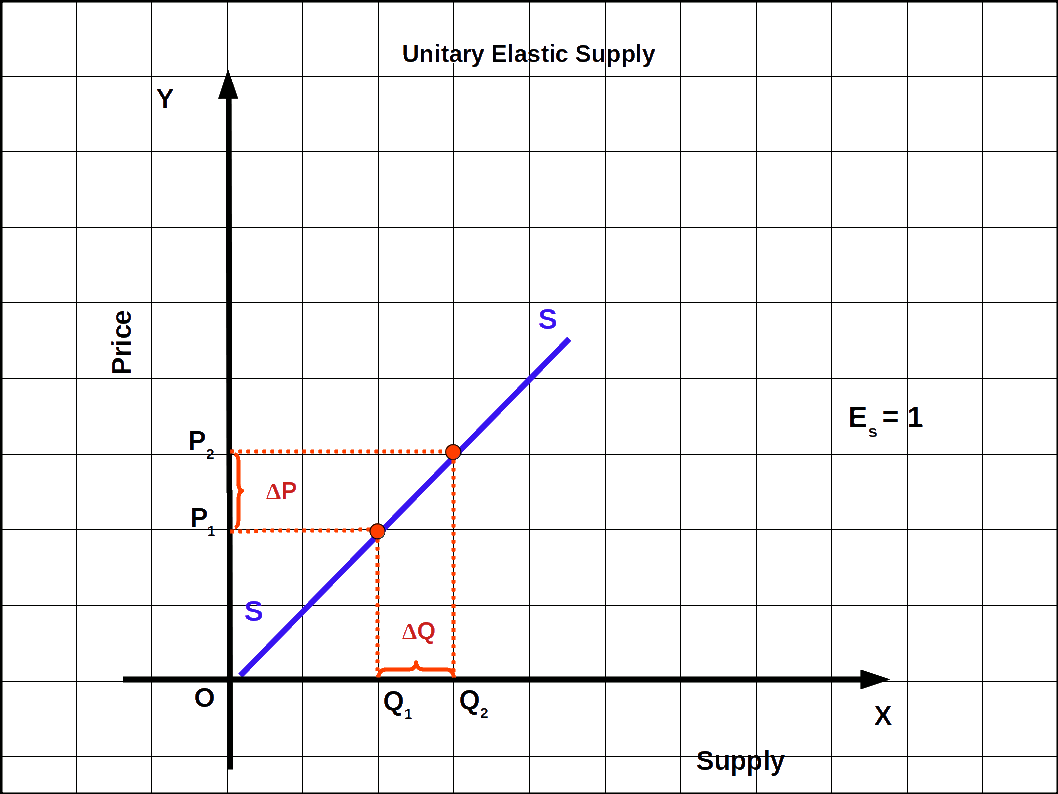
(3) Unitary elastic supply ( es = 1 ) If the percentage change in supply is equal to the percentage change in price it is known as unitary elastic supply. In this case, the supply curve passes through the origin at 45° angle as shown in the below Diagram. The value of elasticity is one.
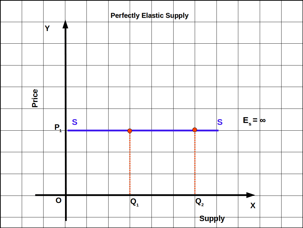
(4) Perfectly elastic supply ( es = ∞ ) When a slight change in price leads to an infinite change in supply, it is called perfectly elastic supply. In such cases, supply curve will be parallel to x-axis as shown in the below Diagram. The value of elasticity would be infinite.
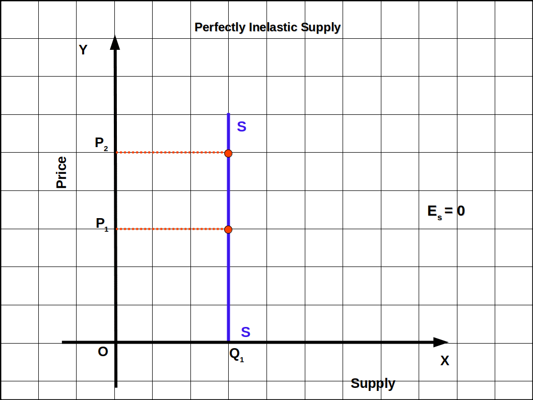
(5) Perfectly inelastic supply ( es = 0 ) Whatever be the changes in price the quantity supplied is unaffected. It is called perfectly inelastic supply. In such case, the supply curve will be parallel to y-axis as shown in the below Diagram. The value of elasticity will be zero.
Methods of Measuring Price Elasticity of Supply Price elasticity of supply is measured in two different ways.
- (1) Percentage method
- (2) Geometric method
(1) Percentage method Under this method price elasticity of supply is measured by dividing the percentage change in quantity supplied by the percentage change in price.
Price elasticity of supply = $$ \mathbf {{\frac{Percentage\,change\, in\, quantity\, supplied}{Percentage\, change\, in\, price}}} $$ $$ \mathbf {e _{s}\,=\,{\frac{{\frac{Change\, in\, quantity\,supplied}{Initial\, quantity}}× 100}{{\frac{Change\, in\, price}{Initial\, price}}× 100}}} $$If p = initial price, q = initial quantity supplied, Δp = change in price and Δq = change in quantity supplied. Then
$$ \mathbf {e \,=\,{\frac{{\frac{Δq}{q}}× 100}{{\frac{ΔP}{P}}× 100}}} $$$$ \mathbf {e \,=\,{{{{\frac{Δq}{q}}}}÷{{{\frac{ΔP}{P}}}}}} $$
$$ \mathbf {=\,{{{{\frac{Δq}{q}}}}×{{{\frac{P}{ΔP}}}}}} $$
$$ \mathbf {e \,=\,{{{{\frac{Δq}{ΔP}}}}×{{{\frac{P}{q}}}}}} $$
The relation between Price and quantity supplied is positive. So the value of elasticity of supply will also be a positive number Similarly the unit of measurement of price and quantity will not affect elasticity.
When the price of a cricket ball was ₹ 10, market supply was 200. When the price increased to ₹ 30, its market supply increased to 1,000. Price elasticity of supply is found as follows: \( \mathbf {e \,=\,{{{{\frac{Δq}{ΔP}}}}×{{{\frac{P}{q}}}}}} \) \( \mathbf {=\,{{{{\frac{800}{20}}}}×{{{\frac{10}{200}}}}}} \) = 2(2) Geometric method If the supply curve is a straight line, extend the supply curve in such a way that it cuts on the x-axis. In the below Diagram, three supply curves are given. The lower part of the curve is extended to x-axis. If we want to find the elasticity at point A on the supply curve, draw a straight line from point A to x-axis. It cuts the x-axis at point Q. In part (a) elasticity at point A is \(e_{s}\, =\,\frac{MQ}{OQ}\) since MQ > OQ \(e_{s}\, =\,\frac{MQ}{OQ}\) > 1. The Supply curve S1 stands for elastic supply. That is, when the supply curve is extended towards the x-axis, if it touches on the negative side of the x-axis, elasticity will be greater than one.
In part (b) at point A elasticity would be \(e_{s}\, =\,\frac{OQ}{OQ}\) = 1. Supply curve S2 stands for unitary elasticity. When supply curve is extended, if it passes through the origin, elasticity would be one. In part (c) elasticity at point A is \(e_{s}\, =\,\frac{MQ}{OQ}\) < 1, which is less than one. Hence MQ < OQ. Supply curve S3 stands for inelastic supply. That is, when supply curve is extended to x-axis, if it cuts the positive Part of x-axis, elasticity would be less than one. If the supply curve is parallel to x-axis the elasticity will be infinite, and if it is parallel to y-axis the elasticity will be zero.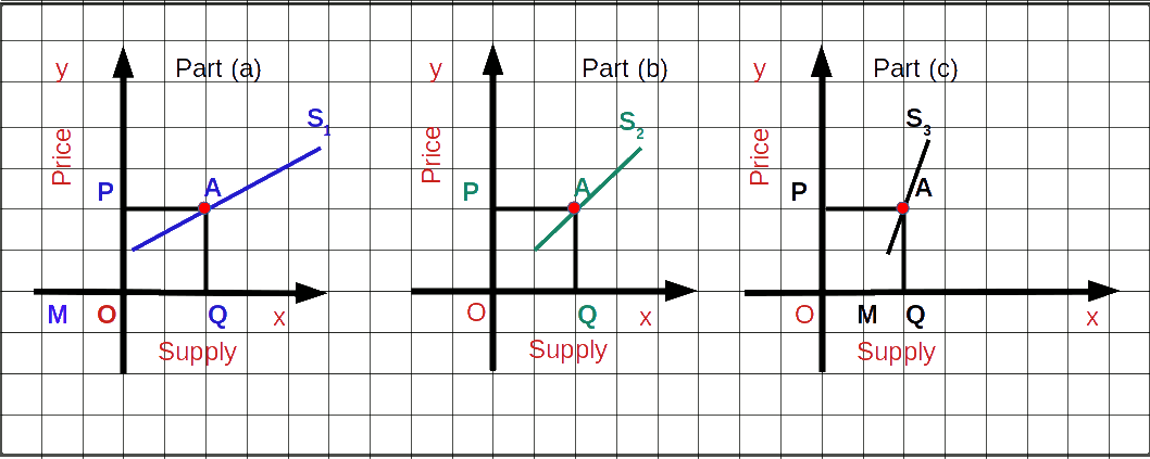
![]()
0 Comments