Plus Two Economics – Chapter 3
Chapter 3:-


An economic unit that produces goods and provides services is called the producer or firm . The producer’s most important aim is to produce goods at least cost thereby maximising his profit. All resources used for production of goods are called inputs. Land, labour, capital and entrepreneurship or organisation are called factor inputs or factors of production.
Goods and services created using inputs are called output. In other words, production is the transformation of inputs into output.
Production Function Product depends on the inputs. Production can take place only if there are inputs. No inputs, no product, no output. In a production unit, when change takes Place in the inputs, quantity of products made in the unit also undergoes change. Output is a function of inputs.
The relationship between inputs and output is called production function. When technology changes, there will be a corresponding change in the quantity of output. Therefore we refer to production function in relation to technology as follows: Using different combinations of various inputs to produce maximum output with a particular technology is called production function. Suppose in a production process there are only two inputs. They are factor 1 and factor 2. If x1 and x2 are the units of factor 1 and factor 2 respectively, q is the quantity of output; production function can be algebraically represented as
\( \mathbf{q\,=\,f(x_1,\,x_2)} \)
| Table 3.1 Production Function | ||||||
|---|---|---|---|---|---|---|
| Factor 2 | X2 | |||||
| Factor 1 | 0 | 1 | 2 | 3 | 4 | |
| x1 | 0 | 0 | 0 | 0 | 0 | 0 |
| 1 | 0 | 1 | 3 | 7 | 10 | |
| 2 | 0 | 3 | 10 | 18 | 24 | |
| 3 | 0 | 7 | 18 | 30 | 40 | |
| 4 | 0 | 10 | 24 | 40 | 50 | |
| 5 | 0 | 12 | 29 | 46 | 56 | |
| 6 | 0 | 13 | 32 | 50 | 57 | |
The table 3.1 gives the various inputs combination and the different quantities of output which can be produced using the inputs. There are two factors in the table: Factor 1 and Factor 2. As we go towards the right, the quantity of factor 2 increases from 0 to 4. As we go down factors the quantity of factor 1 increases from 0 to 6. The shaded area represents quantity of output, q. As combination of inputs change, change also occurs in the quantity of output. If input is 0, output is also 0. As inputs increase output also increases, For example, when factor 1 uses 3 units and factor 2 uses 4 units the output is 40 units.
Isoquant
Isoquant is also known”as equal product curve. Isoquant can be defined as the curve made by joining points of different combinations of two equal output producing inputs. In an isoquant the output at every point will be equal. But the combination of inputs will be different. Look at the below given diagram.
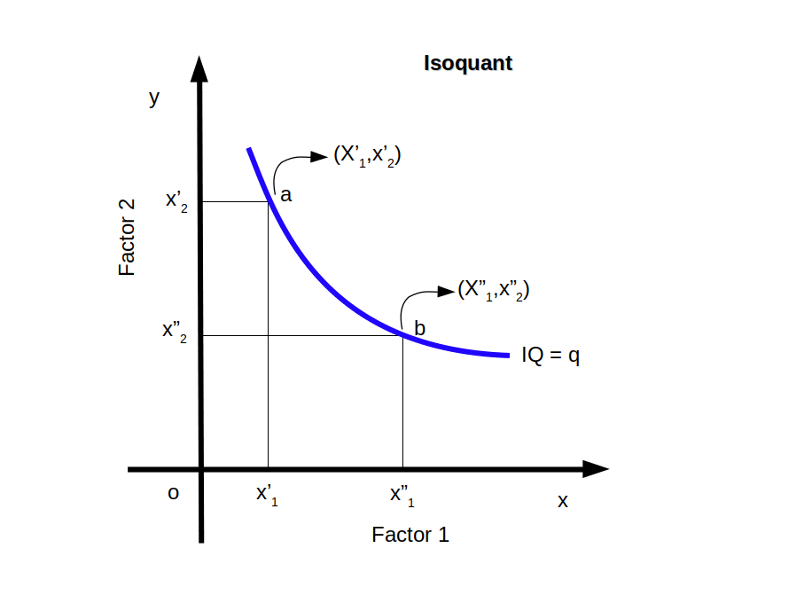 In the diagram, the curve ‘q’ represents an isoquant. In this isoquant, ‘a’ is the point of input combinations where x’1 units of factor 1 and x’2 units of factor 2 are used. Similarly at point ‘b’ factor 1 and factor 2 use x”1 and x”2 units respectively. The output ‘q’ remains unchanged.
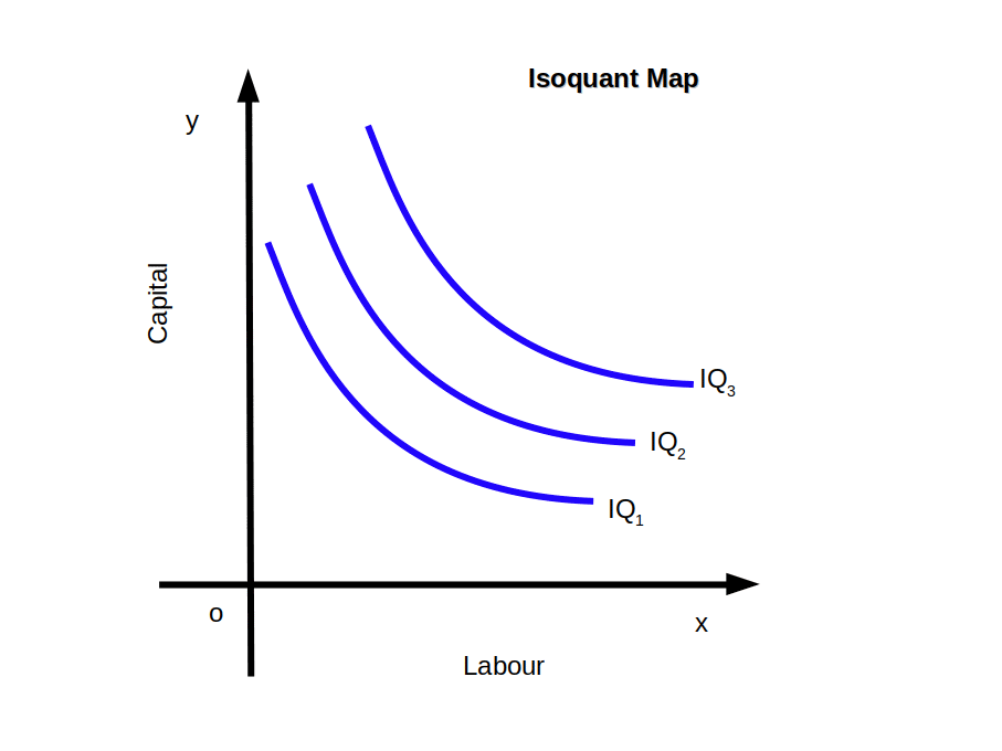
Isoquant Map A group of isoquants is called an isoquant map. Isoquants on the right, represent for more output and those on the left represent less production. Isoquants will be sloping downwards like the indifference curves. Isoquant map is given below.
\( \mathbf{IQ_3\,>\,IQ_2\,>\,IQ_1} \)
Properties of Isoquants Isoquants have the following properties.
- Isoquants are convex to the origin.
- Isoquants slope downwards from left to right.
- Two isoquants will not intersect.
- Higher isoquants represent higher levels of output.
The Short Run and The Long Run One of the important factors that affect production is time period. The time period in production is classified into two (1) Short run and (2) Long run.
Short run is the period in which the firm cannot vary all inputs. The inputs in short run are classified into (1) Variable inputs or Variable factors and (2) Fixed inputs or Fixed factors.
Inputs that can be changed in the short run are called variable inputs. For example, quantity of labour, quantity of raw materials, energy, etc. But all the short run inputs cannot be changed. Such short run inputs which cannot be changed are called fixed inputs. For example, size of the factory building, new machinery, new technology, etc.
Long run is the period in which the firm can vary all inputs. The distinction between fixed inputs and variable inputs is valid only in the short run, In the long run all inputs are variable.
Short Run Production Function The situation in which application of one. factor is varied, while all other factors are kept constant, the production function which operates in such a situation is called short run production function. It is also known as Law of Variable Proportion or Law of Returns to a Factor.
Long Run Production Function The effect of proportionate change in all inputs on output is called Long Run Production Function or Law of Returns to Scale. Since proportion between inputs are fixed, it is also known as Fixed Proportion Production Function.
The production function reflecting the relationship between inputs and output can be explained in terms of total product, average product and marginal product.
Total Product – TP Total product or Total Physical Product (TPP) is the total output produced when a change in quantity of one variable input alone is affected while all other inputs remain constant. Look at Table 3.1. When quantity of factor 2 remains constant and factor 1 increases from 0 to 6, the total product became 0, 1, 3, 7, 10,12 and 13 respectively.
Average Product – AP Average product or Average Physical Product (APP) is the output per unit of variable input. By dividing total product with the number of variable factors we get Average Product.
$$ \mathbf{AP_1 \,=\, {{{\frac{TP}{X_1}} }}} $$
$$ AP_1 \, = \,Average\, Product\, of \,Factor \,1 $$ $$TP\, =\, Total\, Product $$ $$ X_1 \,= \,Amount \,of \,variable \,factor \,used $$
| Table 3.2 Average Product – AP | ||
|---|---|---|
| Quantity of variable factor (X1) | Total Product (TP) | \( \mathbf{AP \,=\, {{{\frac{TP}{X_1}} }}} \) |
| 0 | 0 | Nil |
| 1 | 1 | 1 ÷ 1 = 1 |
| 2 | 3 | 3 ÷ 2 = 1.5 |
| 3 | 7 | 7 ÷ 3 = 2.33 |
| 4 | 10 | 10 ÷ 4 = 2.5 |
| 5 | 12 | 12 ÷ 5 = 2.4 |
| 6 | 13 | 13 ÷ 6 = 2.16 |
Marginal Product – MP Physical Product (MPP) is the addition made to the total product through the addition of one unit of a variable input, keeping all other inputs constant. MP of factor 1 can be written as follows:
$$ \mathbf{MP_1 \,=\, {{{\frac{Change\, in\,TP}{Change \,in\, variable\, input}} }}} $$
$$ or $$
$$ \mathbf{MP_1=\, {{{\frac{ΔTP}{ΔX_1}} }}} $$
where,
$$ΔTP \,= \,Change \,in \,Total \,Product \,and $$ $$ Δx_1 \,= \,Change \,in \,Variable \,Input $$ $$ or $$ $$ \mathbf{MP_n\, = \, TP_n\,-\,TP_{n-1}} $$
“n” is the number of units of variable input employed
| Table 3.3 Marginal Product – MP | ||
|---|---|---|
| Quantity of variable factor (X1) | Total Product (TP) | \( \mathbf{MP \,=\, {{{\frac{ΔTP}{ΔX_1}} }}} \) |
| 0 | 0 | Nil |
| 1 | 1 | 1 ÷ 1 = 1 |
| 2 | 3 | 2 ÷ 1 = 2 |
| 3 | 7 | 4 ÷ 1 = 4 |
| 4 | 10 | 3 ÷ 1 = 3 |
| 5 | 12 | 2 ÷ 1 = 2 |
| 6 | 13 | 1 ÷ 1 = 1 |
| Table 3.4 Marginal Product – MP | ||
|---|---|---|
| Quantity of variable factor (X1) | Total Product (TP) | \( \mathbf{MP_n\, = \, TP_n\,-\,TP_{n-1}} \) |
| 0 | 0 | Nil |
| 1 | 1 | 1 – 0 = 1 |
| 2 | 3 | 3 – 1 = 2 |
| 3 | 7 | 7 – 3 = 4 |
| 4 | 10 | 10 – 7 = 3 |
| 5 | 12 | 12 – 10 = 2 |
| 6 | 13 | 13 – 12 = 1 |
Laws of Returns (Production) We have already understood that output is the function of inputs under given technology. More the inputs, more will be quantity of output produced. Change in quantity of output may be referred to as ‘return’. Law of Returns (or production) explains the change in output as a result of change in inputs.
An example will clarify this. If a firm wants to increase its production (output) to meet growing demand of its product, it can do so either by increasing inputs or by changing technology. Keeping the technology constant, output can be increased by increasing the quantity of inputs. For instance, if a firm manufacturing 100 TV sets daily wants to double its production, it has to increase inputs accordingly. But here one difficulty arises. It is not possible for the firm to increase all inputs at a short notice. During the short period, although the firm can increase variable inputs (like raw materials, labour, power, etc.), it cannot change the size of fixed inputs (like machines, building, etc.). Thus, there are two situations—one, when only variable factors can be changed keeping the fixed factors constant (short period) and two, when all the factors can be changed (long period). The law operating in the first situation is called Law of Variable Proportion since proportion (or ratio) between fixed factors and variable factors is changed. This law is also termed as Returns to a Factor because application of one factor is varied while keeping all other factors constant. As against this, the law which operates in the second situation (long period) is called Law of Returns to Scale since the whole scale of production is changed by changing all the factors in the same proportion. The following chart further clarifies the position.

The Law of Diminishing Marginal Product and the Law of Variable Proportion The law of diminishing marginal product is short run production function. In the short run, the producer can change the quantity of output only by changing the quantity of variable factors.
If we increase the employment of an input, keeping other inputs constant, eventually, a point will be reached after which the resulting marginal product starts falling. This is called the law of diminishing marginal product or returns to a factor.
A related concept of the law of diminishing marginal product is the law of variable proportions.
The law of variable Proportion states that when more and more units of a variable factor are added with fixed factors, initially TP increases at an increasing rate, then increases at a diminishing rate and finally starts to decline. If we express in terms of MP, the law states that when the quantities of a variable factor are added with fixed factors, initially MP increases, then falls and finally becomes negative.
Law of diminishing marginal product and the law of variable proportion are one and the same. When more and more units of variable factors are added to constant factors, total product and marginal product pass through three stages.
They are:
Stage 1 – Increasing Returns to a Factor
Stage 2 – Diminishing Returns to a Factor
Stage 3 – Negative Returns to a Factor
| Table 3.5 | |||
| Quantity of variable factor | Total Product (TP) | Average Product (AP) | Marginal Product (MP) |
|---|---|---|---|
| 1 | 10 | 10 | 10 14 15 17 |
| 2 | 24 | 12 | |
| 3 | 39 | 13 | |
| 4 | 56 | 14 | |
| 5 | 70 | 14 | 14 8 6 0 |
| 6 | 78 | 13 | |
| 7 | 84 | 12 | |
| 8 | 84 | 10.5 | |
| 9 | 81 | 9 | -3 -5 |
| 10 | 76 | 7.6 | |
We shall discuss these three stages with the help of production function.
Stage I : Increasing Returns to a Factor
In the first stage, TP increases at an increasing rate. Then MP also increases and reaches. its maximum, AP increases. The first stage ends when AP is maximum. This stage represents Increasing returns to a factor.
Stage II : Diminishing Returns to a Factor
In the second stage, TP increases at a decreasing rate. Here, MP falls and becomes zero, AP declines. This stage represents Diminishing returns to a factor.
Stage III : Negative Returns to a Factor
In the third stage, TP starts declining. Then MP becomes negative. AP continues to decline, but never becomes zero. This stage represents Negative returns to a factor.
 Relation among variable inputs and TP, MP and AP are given in the above Graph. Total product curve first increases and then decreases. Similarly MP first increases, then decreases and finally becomes negative. AP continuously declines.

| Table 3.6 Short Run Production Function | ||
| Stage I Increasing Returns to a Factor |
Stage II Diminishing Returns to a Factor |
Stage III Negative Returns to a Factor |
| TP increases at an increasing rate | TP increases at a diminishing rate | TP starts declining |
|---|---|---|
| AP increases | AP declines | AP declines but never becomes zero |
| MP increases and reaches its maximum | MP falls and becomes zero | MP becomes negative |
Relation between TP and MP
- When TP increases at an increasing rate, MP increases upto variable factor x1 as in the above Diagram.
- When TP increases at a decreasing rate, MP decreases but remains positive from the variable factor x1 to x1‘ in the above Diagram.
- When TP reaches its maximum, MP becomes zero. See variable factor x1‘ in the above Diagram.
- When TP decreases MP becomes negative after the variable factor x1‘ as in the above Diagram.
Relation between MP and AP
- As AP increases, MP is greater than AP. In the above Diagram, till variable input x1, AP curve increases. Then MP curve is above the AP curve.
- When AP reaches maximum, AP and MP will be equal. In the above Diagram, when variable input is x1, AP is equal to MP.
- When AP decreases, MP is less than AP after variable factor x1. This is shown in the above Diagram.
Returns to Scale Returns to scale is a long-run production function. In the long run, there is no distinction between fixed factors and variable factors. In the long run all factors are variable. Returns to scale refers to change in output caused by proportionate change in all inputs. Hence the input ratios remain the same.
It is possible to change output in the long run by changing all inputs simultaneously. When all inputs are changed in the same proportion, TP responds in three different ways. They are:
Increasing Returns to Scale (IRS)
Constant Returns to Scale (CRS)
Diminishing Returns to Scale (DRS)
1. Increasing Returns to Scale – IRS: When the percentage change in output is more than the percentage change in input, it is called Increasing Returns to Scale. It is a situation when proportionate increase in all inputs result in more than proportionate increase in output.
In the following table when inputs are increased by 100 per cent, the output increased by 150 percent. In other words, if input is doubled, output will be more than doubled.
| Table 3.7 Short Run Production Function | |||||
| Factor 1 (X1) | Factor 2 (X2) | Ratio between factors (X1: X1) | Total Product (q) | Increase in Input (%) | Increase in Total Product (%) |
| 2 | 3 | 2 : 3 | 10 | — | — |
|---|---|---|---|---|---|
| 4 | 6 | 2 : 3 | 25 | 100 | 150 |
| 8 | 12 | 2 : 3 | 55 | 100 | 120 |
2. Constant Returns to Scale – CRS: When the percentage change in output is equal to percentage change in input, it is called Constant Returns to Scale. It is a situation when proportionate increase in input becomes equal to proportionate increase in output.
In the following table when input increased by 100, the output also increased by 100. In other words, if input is doubled, output also will be doubled.| Table 3.8 Short Run Production Function | |||||
| Factor 1 (X1) | Factor 2 (X2) | Ratio between factors (X1: X1) | Total Product (q) | Increase in Input (%) | Increase in Total Product (%) |
| 2 | 3 | 2 : 3 | 10 | — | — |
|---|---|---|---|---|---|
| 4 | 6 | 2 : 3 | 20 | 100 | 100 |
| 8 | 12 | 2 : 3 | 40 | 100 | 100 |
3. Diminishing Returns to Scale – DRS: When the percentage change in output is less than the percentage change in inputs, it is called Diminishing Returns to Scale. It is a situation in which proportionate increase in inputs causes less than proportionate increase in output.
In the following table when input is increased by 100 per cent, output is increased by 50 per cent. In other words, if inputs are doubled the output will be less than doubled.| Table 3.9 Short Run Production Function | |||||
| Factor 1 (X1) | Factor 2 (X2) | Ratio between factors (X1: X1) | Total Product (q) | Increase in Input (%) | Increase in Total Product (%) |
| 2 | 3 | 2 : 3 | 10 | — | — |
|---|---|---|---|---|---|
| 4 | 6 | 2 : 3 | 15 | 100 | 50 |
| 8 | 12 | 2 : 3 | 20 | 100 | 33.3 |
Cobb-Douglas Production Function C.W. Cobb and Paul H. Douglas conducted studies in a few factories in America. On the basis of their studies they formulated a production function named – Cobb-Douglas production function and it is represented as \( \mathbf{q\, = \, x{_1^α}x{_2^β}} \). Here, q is quantity of output, x1 is the quantity of factor 1, x2 is the quantity of factor 2, α and β are constants.
$$ \mathbf{{ q\, = \, {(t\overline{x}_1){^α}(t\overline{x}_2){^β}}}} $$ $$\mathbf{=\,t^{α+β} \,\, {{\overline{x}_1{^α}} \,\, {\overline{x}_2{^β}}}} $$ If α + β = 1 production function is CRS.
If α + β > 1 production function is IRS.
If α + β < 1 production function is DRS.
\( \mathbf{q\, = \, 5\,×\,3{^2}\,× 2{^4}} \) = 5 × 9 × 16 = 720
Here α = 2, β = 4
∴ α + β = 2 + 4 = 6 > 1
So, production function is IRS.
\( \mathbf{q\, = \, 25\,×\,100{^.75}\,× 100{^.25}} \) = 25 × 100.75 + .25 = 25 × 100 = 2500
Here α = .75, β = .25
∴ α + β = .75 + .25 = 1
So, production function is CRS.
Costs Costs refer to the expenses incurred by the producer to produce goods and services. Wages, rent, interest, insurance premium, electricity charges, cost of raw material, transportation, wear and tear, expenses for training employees, etc., are examples of costs.
Short Run Costs We saw that in short run Production function, some factors are constant while others are variable. So, in the short run, costs can be classified as Total Fixed Cost (TFC) and Total Variable Cost (TVC). In the long run, all costs are variable.
Total Fixed Cost – TFC: The total cost incurred by the producer for the purchase of fixed inputs is called Total Fixed Cost, In the short run, fixed costs are the costs which do not change with the change in quantity of output. Therefore, cost that does not change with the change in output is called fixed cost. Rent for land and buildings, salary of permanent staff, interest on loans, insurance premium, etc., are examples of fixed costs.
Total Variable Cost – TVC: The total cost incurred by the producer on variable inputs is called Total Variable Cost. These costs change as the quantity of output changes. Therefore, cost that changes with change in quantity of output is called Total Variable Costs. If the quantity of output increases or decreases variable cost will increase or decrease accordingly. When production becomes zero, variable cost also becomes zero. Cost of raw materials, energy cost, transportation cost, salary of temporary employees, etc., are examples of variable costs.
Total Cost – TC: Total cost is the sum total of all costs incurred by the producer to produce goods and services. It is the sum of total fixed costs and total variable costs.
$$ \mathbf{TC \,= \,TFC\, + \,TVC} $$ The difference between TFC and TVC exists only in the short run. In the long run, all costs are variable. If output is zero, TC will be equal to TFC. Total cost changes in Proportion to variable cost.
| Table 3.10 Cost Function | |||
|---|---|---|---|
| q | TFC | TVC | TC |
| 0 | 20 | 0 | 20 |
| 1 | 20 | 10 | 30 |
| 2 | 20 | 19 | 39 |
| 3 | 20 | 27 | 47 |
| 4 | 20 | 34 | 54 |
| 5 | 20 | 40 | 60 |
| 6 | 20 | 45 | 65 |
| 7 | 20 | 49 | 69 |
| 8 | 20 | 54 | 74 |
| 9 | 20 | 60 | 80 |
| 10 | 20 | 67 | 87 |
| 11 | 20 | 75 | 95 |
| 12 | 20 | 84 | 104 |
| 13 | 20 | 94 | 114 |
To increase output, the firm has to bring more variable inputs. As a result TVC and TC will increase. So, in the short run, when output increases TC and TVC increase. Table 3.10 shows the cost function of a firm.
In the Table 3.10, when output is 0, TFC is 20. When output becomes 13 units TFC remains at 20. There is no change in TFC. Moreover, when output is zero, TFC and TC are equal. At zero output level, TVC is zero. When output increases, TVC and TC increase.
Shape of TFC, TVC and TC Curves In the below given Diagram, output is marked on the x-axis and cost on the y-axis. TFC curve is parallel to x-axis. TVC curve starts from the origin because when output is zero TVC is also zero. Both TVC and TC curves are sloping upwards. They have an inverted ‘S’ shape.
 TVC curve starts from 0 and slowly increases, then rises rapidly, along with the output. When output is 0, TVC is also 0. TC curve begins from point F where TFC curve cuts the y-axis. TC initially increases slowly and then rises rapidly as output increases.
Below given graph shows the TFC, TVC and TC curves drawn with the data given in Table 3.10.
Average Variable Cost – AVC Average variable cost is the variable cost per unit of output. AVC is calculated by dividing the TVC by the number of units of output.
$$ {AVC \,=\, {{{\frac{TVC}{q}} }}} $$ $$∴\, TVC \, =\, q.AVC $$
Average Fixed Cost – AFC Average fixed cost is the fixed cost per unit of output. AFC is calculated by dividing the TFC by the number of units of output.
$$ {AFC \,=\, {{{\frac{TFC}{q}} }}} $$ $$∴\, TFC \, =\, q.AFC $$
Short Run Average Cost – SAC Cost per unit of output in the short run is called short run average cost. SAC is usually called Average Cost (AC). If total cost is divided by the number of units of output, we get SAC.
$$ {SAC \,=\, {{{\frac{TC}{q}} }}} $$ $$∴\, TC \, =\, q.SAC $$
It is the sum of AFC and AVC, ie., SAC = AFC + AVC
Then,
SAC = AFC + AVC = 10 + 25 = ₹35
Short Run Marginal Cost – SMC Short Run Marginal Cost is defined as the change in total cost per unit of change in output.
$$ {SMC \,=\, {{{\frac{Change \,in \,Total \,Cost}{Change \,in \,Output}} }}} \, = \,{ {{{\frac{ΔTC}{Δq}} }}}$$ $$ or $$ $$ SMC_n \, =\, TC_n\, – \, TC_{n-1} $$ $$ or $$ $$ SMC \, =\, [TC\,of\,q_1\,unit]\, – \, [TC \,of\,q_{1}\,-\,1 \,unit] $$

\( \mathbf{TC \,= \,TFC \,+ \,TVC}\)
\( or \)
\( \mathbf{TC \,= \,AC \,× \,q }\)
\( \mathbf{TFC \,= \,TC \,- \,TVC }\)
\( or \)
\( \mathbf{TFC \,= \,AFC \,× \,q}\)
\( \mathbf{TVC \,= \,TC \,- \,TFC}\)
\( or \)
\( \mathbf{TVC \,= \,AVC \,× \,q}\)
\( \mathbf{AC \,= AFC \,+ \,AVC}\)
\( or \)
\( \mathbf {AC\,=\, {\frac{TC}{q}}} \)
\( \mathbf{AFC \,= \,AC \,- \,AVC}\)
\( or \)
\( \mathbf {AFC\,=\, {\frac{TFC}{q}}} \)
\( \mathbf{AVC \,= \,AC \,- \,AFC}\)
\( or \)
\( \mathbf {AVC\,=\, {\frac{TVC}{q}}} \)
\( \mathbf {MC_n \,= \,TC_n \,- \,TC_{n – 1}}\)
\( or \)
\( \mathbf {MC\,=\, {\frac{ΔTC}{Δq}}} \)
Average Fixed Cost Curve (AFC Curve) At all levels of output TFC is constant. So when output increases AFC will decrease continuously. See Table 3.6. So, the shape of AFC curve will be rectangular hyperbola as shown in the below Diagram. AFC curve decreases and approaches to 0; but it will never be 0.
If we know AFC, we can find TFC by multiplying AFC with q. That is
\( TFC = AFC × q \)
 In the above Diagram, when the quantity of output became OQ, AFC is OA. So, TFC at Q level is
TFC = AFC x q = OA × OQ = OAFQ, the shaded area.
| Table 3.11 Short Run Cost | |||||||
|---|---|---|---|---|---|---|---|
| q | TFC | TVC | \(\mathbf{TFC \,+ \,TVC \,= \,TC}\) | \( \mathbf {AFC\,=\, {\frac{TFC}{q}}} \) | \( \mathbf {AVC\,=\, {\frac{TVC}{q}}} \) | \( \mathbf {SAC\,=\, {\frac{TC}{q}}} \) | \( \mathbf {MC_n \,= \,TC_n \,- \,TC_{n – 1}}\) |
| 0 | 20 | 0 | 20 | – | – | – | – |
| 1 | 20 | 6 | 26 | 20 | 6.0 | 26.0 | 6 (= 26 – 20) |
| 2 | 20 | 11 | 31 | 10 | 5.5 | 15.5 | 5 (= 31 – 26) |
| 3 | 20 | 15 | 35 | 6.66 | 5 | 11.66 | 4 ( = 35 – 31) |
| 4 | 20 | 18 | 38 | 5 | 4.5 | 9.5 | 3 (= 38 – 35) |
| 5 | 20 | 20 | 40 | 4 | 4.0 | 8.0 | 2 (= 40 – 38) |
| 6 | 20 | 21 | 41 | 3.33 | 3.5 | 6.83 | 1 (= 41 – 40) |
| 7 | 20 | 23 | 43 | 2.86 | 3.28 | 6.14 | 2 (= 43 – 41) |
| 8 | 20 | 26 | 46 | 2.50 | 3.25 | 5.75 | 3 (= 46 – 43) |
| 9 | 20 | 30 | 50 | 2.22 | 3.33 | 5.55 | 4 (= 50 – 46) |
| 10 | 20 | 35 | 55 | 2.00 | 3.50 | 5.50 | 5 (= 55 – 50) |
| 11 | 20 | 41 | 61 | 1.80 | 3.72 | 5.52 | 6 (= 61 – 55) |
In Table 3.11 when output q is 5 units AFC is ₹ 4. Then TFC = 4 × 5 = 20. On the basis of Table 3.11 AFC curve is drawn in the below Graph.
Average Variable Cost Curve (AVC Curve) As the quantity of output increases AVC initially decreases and later increases. The AVC is a ‘U’ shaped curve.
 Above given Diagram shows the AVC curve. If we know AVC and the quantity of output we can calculate TVC. TVC = AVC × q. In the diagram, when output becomes OQ, AVC is OV. So, TVC = AVC × q = OV × OQ = OVCQ.The shaded area in the diagram.
In Table 3.11, when output is 3 units, AVC is ₹ 5. Then, TVC = AVC × q = 5 × 3 = ₹ 15.
Short run Average Cost Curve – (SAC Curve) Initially, as the output increases SAC decreases and later it increases. This is shown in Table 3.11. So the SAC curve assumes U shaped cure. Below given Diagram shows short run average cost curve.
 From SAC we can calculate TC. To find the TC of an output at a particular level, multiply SAC with the quantity of output. That is, TC = SAC × q = OA × OQ = OACQ.The shaded area in the diagram.
In Table 3.11 when output is 10 units SAC is ₹ 5.5. Then TC =SAC × q = 5.5 × 10 = ₹ 55.
Short Run Marginal Cost Curve (SMC Curve)
SMC curve initially falls as output rises and later increases. This can be seen in Table 3.11. So SMC is a “U” shaped curve as shown in the below Diagram.
 The slope of TC or TVC is SMC. When TC and TVC increase at a diminishing rate SMC decreases. When they increase at an increasing rate SMC increases. This is shown in Table 3.11.
AVC, SAC and SMC are drawn in the below given Graph based on Table 3.11. Here AVC, SAC and SMC curves are “U” shaped.
Relationship between AVC and MC
- AVC and MC initially falls and later rise.

- When AVC falls, MC will be less than AVC.
- When AVC rises, MC will be more than AVC.
- When AVC is minimum, MC and AVC will be equal. In the diagram when output is q, AVC = MC. MC cuts the minimum point of AVC from below.
Relationship between SAC and AVC
- At a given level of output the difference between SAC and AVC curves will be equal to the AFC of that output.
- The difference between SAC and AVC decreases as the output increases.
- The minimum point of AVC curve is on the left of the minimum point of SAC.
Long Run Costs In the long run, all inputs are variable. Therefore, there is no distinction between fixed cost and variable cost. The costs incurred for all inputs in the long run are called Long Run Total Cost. Long Run Average Cost (LRAC) and Long Run Marginal Cost (LRMC) are Long Run Costs.
\( \mathbf {LRAC\,=\, {\frac{TC}{q}}} \)
\( \mathbf {LRMC\,=\, {\frac{ΔTC}{Δq}}} \)
Shapes of Long Run Cost Curves
LRAC and LRMC curves are U shaped. Both are flatter than SAC curve. LRAC and LRMC initially decrease and then increase. More over, their centre would be comparatively flat. The U-shape of these curves is caused by the returns to scale. LRAC curve and LRMC curve are shown in below Diagram.
 LRAC and LRMC initially decrease because of increasing returns to scale. The middle of LRAC and LRMC is flat due to the constant returns to scale. LRMC curve cuts at the minimum point of LRAC from below, LRAC and LRMC increase due to the diminishing returns to scale.
Relationship between LRAC and LRMC
- When LRAC falls LRMC is less than LRAC.
- When LRAC rises LRMC is more than LRAC.
- LRMC curve cuts LRAC curve at the minimum Point from below.
- Minimum point of LRMC will be on the left of LRAC.
- As per traditional theory of cost, LRAC and LRMC curves are U shaped.
![]()
0 Comments