Plus Two Economics Chapter 2
Chapter 2:-


Introduction: The theory of consumer behaviour analyses how a consumer maximises his satisfaction from his consumption expenditure.
 Consumers buy or demand goods and services to satisfy their wants. They. can satisfy their wants by consuming goods. Goods are bought by consumers to reach the highest level of satisfaction, i.e., consumer’s equilibrium. Consumers have to decide what quantity of a good they should buy at a given price and at a given point of time. In other words, we have to study consumer behaviour. To understand consumer behaviour, first we have to understand the concept utility. Utility is the want Satisfying power of a commodity or service. There are three important theories that explain the measurement of utility and the process that leads to consumer’s equilibrium. They are:
- Cardinal utility approach of Alfred Marshall
- Ordinal utility approach of J. R. Hicks
- Revealed preference Hypothesis of Paul A. Samuelson


Here we discusses how a consumer achieves consumer’s equilibrium according to the ordinal utility approach. Ordinal utility approach is also known as Indifference curve approach.
Consumption Bundle
A consumer cannot buy every thing he/she wants. Since wants are unlimited, he/she has to make a choice. Normally consumers buy many goods. But for ease of analysis let us assume that there are only two goods. They are good 1 and good 2. Any combination of the amount of two goods is called a consumption bundle. Let x1 be the amount of good 1 and x2 amount of good 2. (x1, x2) can be called consumption bundle.
 Bundle (4, 6) contains 4 units of good 1 and 6 units-ef good 2. Similarly, bundle (10, 15) contains 10 units of good 1 and 15 units of good 2.
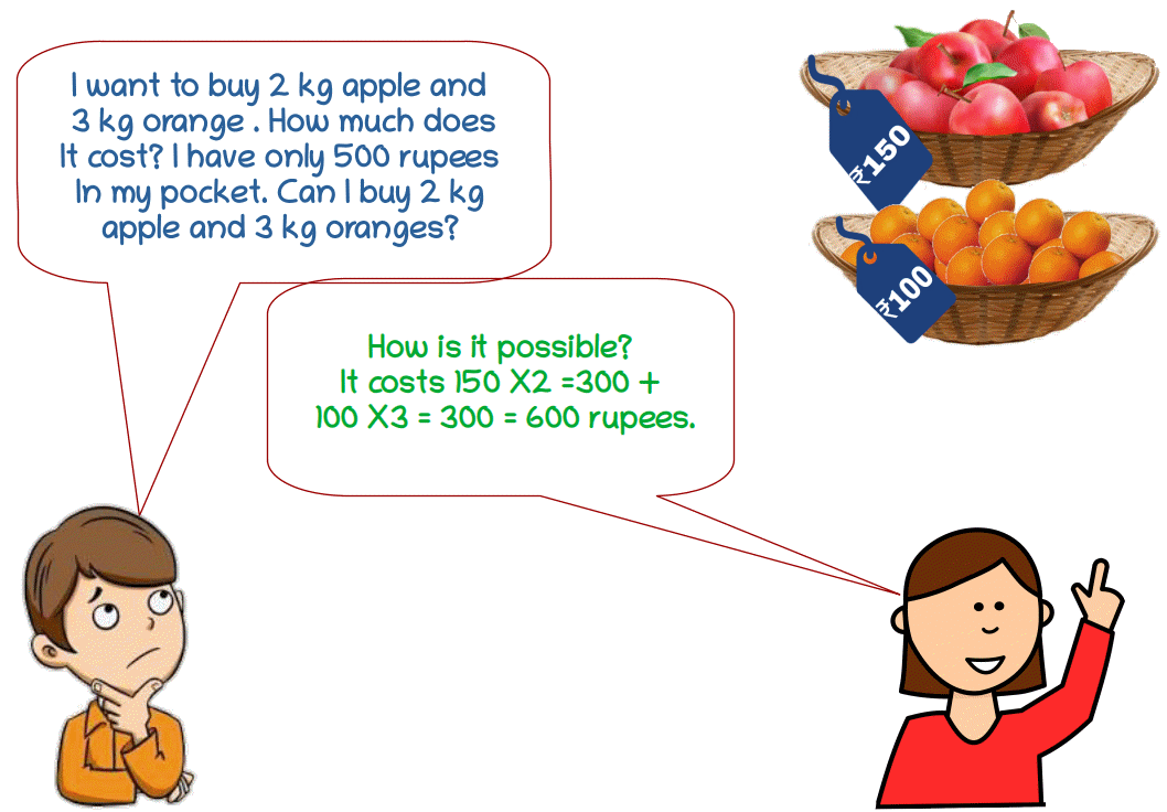
Consumer’s Budget
Consumer’s budget is the income or amount of money available for spending on either goods as he wishes. The consumer can spend his entire income either on good 1 or on good 2 or combination of both. ‘Consumer’s budget is the money income of the consumer which he can use to buy goods and services.
To buy sugar and tea Sindhu has ₹100 and Sethu has ₹75. Let us Find Sindhu’s and Sethu’s budget. Here we can say that Sindhu’s budget is ₹100 and Sethu’s budget is ₹75.
Budget Set
A set of consumption bundles is known as budget set. In other words, it is defined as the collection of all the bundles that the consumer can buy with his income at the prevailing market prices.
Consumer’s behaviour is constrained by his budget. His expenditure should be less than or equal to his budget. Budget constraint can be defined algebraically as P1x1 + P2x2 ≤ M, where, P1 = Price per unit of good 1, P2 = Price per unit of good 2, x1 = Number of units of good 1, x2 = Number of units of good 2 and M = Money income available to the consumer. The inequality P1x1 + P2x2 ≤ M is called Consumer’s Budget Constraint.
Budget Constraint = \( \mathbf{{{P_1 X_1 + P_2 X_2 ≤ M} }} \)
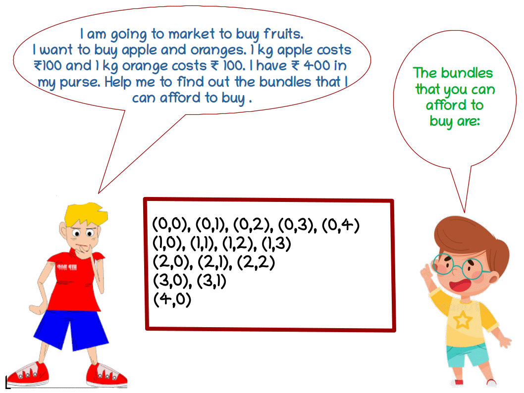
 Let us explain this using an example. Suppose a consumer has ₹20 to spend on two goods. The price per unit of good 1 and good 2 is ₹5. Then the budget set equation is 5x1 + 5x2 ≤ 20. As per this budget set of consumer, the following are the available bundles of good 1 and good 2 which cost less than or equal to ₹20.
{(0, 0), (0, 1), (0, 2), (0, 3), (0, 4), (1, 0), (1, 1), (1, 2), (1, 3), (2, 0), (2, 1), (2, 2), (3, 0), (3, 1), (4, 0)}
These bundles can be plotted in a graph.
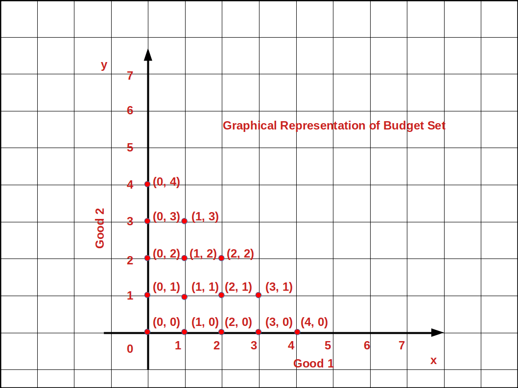 In the above given graph, bundles (0, 4) (1, 3) (2, 2) (3, 1) and (4, 0) are cost exactly equal to ₹20. All other bundles cost less than ₹20.
Budget Line
Budget line is defined as the locus of points of combinations of good 1 and good 2 which cost exactly equal to income. In other words, budget line is the line which consists of all the bundles or combinations that cost exactly equal to the consumer’s income. Algebraically,
Budget Line = \( \mathbf{{{P_1 X_1 + P_2 X_2 = M} }} \)
If the consumer spends his entire income on good 1, he can buy \( \mathbf {{{{\frac{M}{P_1}} }}} \) units of good 1. On the contrary, if he spends the entire income on good 2 he can buy \( \mathbf {{{{\frac{M}{P_2}} }}} \) units of good 2.
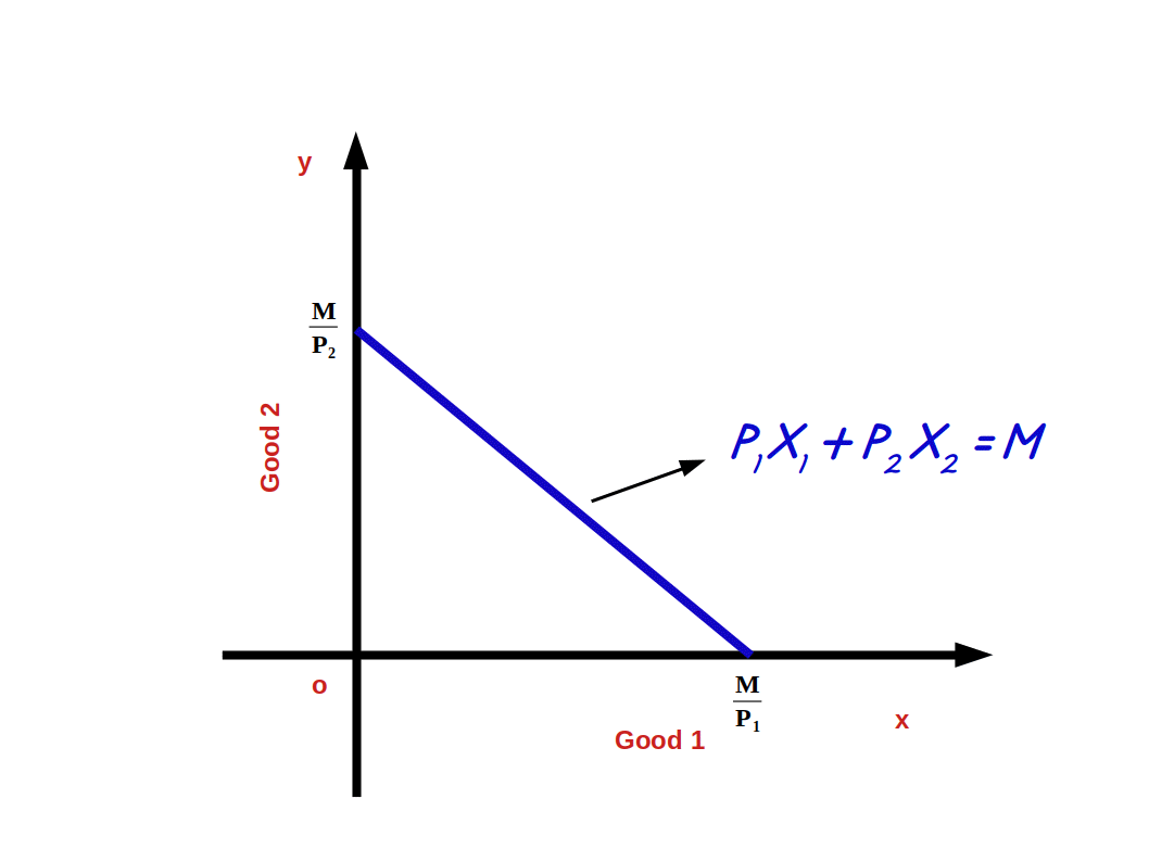
If we represent good 1 on x-axis and good 2 on y-axis, \( \mathbf {{{{\frac{M}{P_1}} }}} \) (the point where budget line touches x-axis) becomes the horizontal intercept and \( \mathbf {{{{\frac{M}{P_2}} }}} \) (the point where budget line touches y-axis) becomes vertical intercept as shown in above diagram.
How to find Horizontal intercept and Vertical intercept ?
Consider the budget line P1x1 + P2x2 = M
If x2 = 0 ie., the consumer does not buy good 2, the quantity of x1 would be:
P1x1 + P2 × 0 = M
P1x1 = M
\( \mathbf {x_1 \, = \, {{{{\frac{M}{P_1}}} }}} \) or \( \mathbf{( {{{{\frac{M}{P_1}}, 0 ) } }}} \) is the horizontal intercept. This is the point where budget line touches x-axis.
If x1 = 0 i.e., the consumer does not buy good 1, the quantity of x2 is
P1 × 0 + P2x2 = M
P2x2 = M
\( \mathbf {x_2 \, = \, {{{{\frac{M}{P_2}}} }}} \) or \( \mathbf{(0, {{{{\frac{M}{P_2}} ) } }}} \) This is the vertical intercept where budget line touches y-axis.
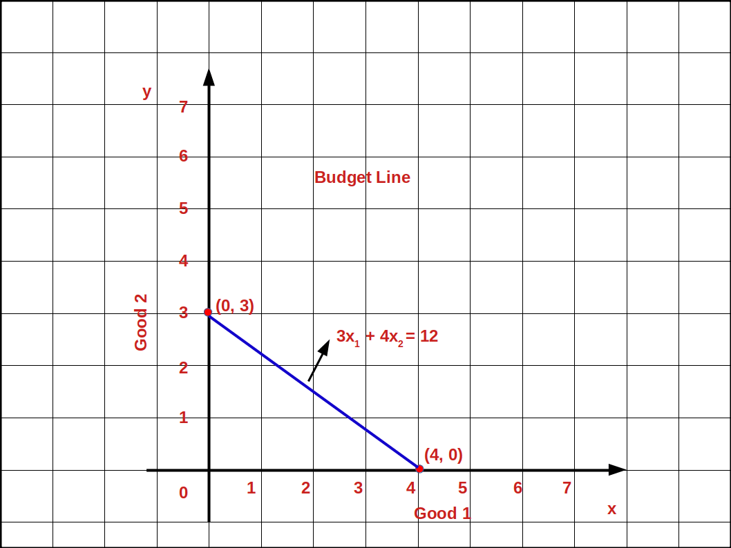
Let us practice an example. In the budget line equation
3x1 + 4x2 = 12, if X2 = 0
3x1 + 4 × 0 = 12,
3x1 = 12
x1 = \( \mathbf {{{{\frac{12}{3}} }}} = 4 \) is the horizontal intercept, i.e., (4, 0).
if x1 = 0, 3 × 0 + 4x2 = 12
4x2 = 12
x2 = \( \mathbf {{{{\frac{12}{4}} }}} = 3 \) is the vertical intercept., i.e., (0, 3)
The budget line 3x1 + 4x2 = 12 is shown in the below graph.
There is an another method to find budget line equation.
Solve the equation P1x1 + P2x2 = M for x2
i.e., P2x2 = M – P1x1
x2 = \( {{{{\frac{M – P_1x_1}{P_2}} }}} \)
x2 = \( {{{{{\frac{M}{P_2}}} – {\frac{P_1}{P_2}} }}} x_1\)
\( {\frac{M}{P_2}} \) is the vertical intercept, \( – {\frac {P_1}{P_2}} \) is the slope of the budget line.
Let us practice an example. Consider the budget line equation 5x1 + 5x2 = 20
When we solve for x2
5x1 + 5x2 = 20
5x1 + 5x2 = 20 – 5x1
x2 = \( {{{{\frac{20 – 5x_1}{5}} }}} \)
= \( {{{{{\frac{20}{5}}} – {\frac{5x_1}{5}} }}} \)
x2 = 4 – x1
In this form of the budget line the vertical intercept is 4 and the slope is -1.
The Table 2.1 shows the different bundles that can be bought with = 20 using the equation x2 = 4 – x1.
| Table 2.1 | ||
| x1 | x2 = 4 – x1 | Bundles |
|---|---|---|
| 0 | 4 – 0 = 4 | (0, 4) |
| 1 | 4 – 1 = 3 | (1, 3) |
| 2 | 4 – 2 = 2 | (2, 2) |
| 3 | 4 – 3 = 1 | (3, 1) |
| 4 | 4 – 4 = 0 | (4, 0) |
In the below Graph we have different bundles of (0, 4) (1, 3) (2, 2) (3, 1) (4, 0).
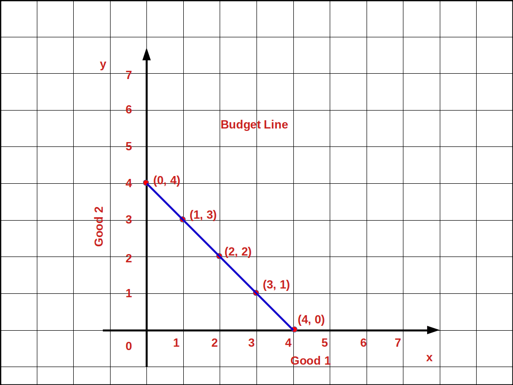
When these bundles are joined with a line, it is called budget line. The cost of all these bundles is exactly equal to the consumer’s income of ₹20.
Points on, above and below the Budget line
In any of the bundles or points below the budget line the consumer does not spend all his income. He has some money unused. Using this amount he can buy more units of good 1 or good 2 or both.
In the above Diagram points A, B, C are on the budget line. Point D is below the budget line and point E is outside the budget line. At point A he buys 1 unit of good 1 and 3 units of good 2 (1, 3). At point B he buys 2 units of good 1 and 2 unit of good 2 (2, 2) and at point C he can buy 3 units of good 1 and 1 unit of good 2 (3, 1). The bundles A B and C are known as efficient bundles. But at point D he buys 1 unit of good 1 and 1 unit of good 2 (1, 1). Then his expenditure at point D will be less than his income. This bundle is called inferior bundle. But point E is outside the budget line. To buy goods at this point the consumer’s income will not be enough. But this bundle would be superior to the bundle on the budget line. This bundle is known as superior bundle or preferred bundle.

- Any point on budget line indicates combinations of good 1 and good 2 a consumer can purchase which cost an amount exactly equal to his income. This bundle is known as efficient bundle.
- Any point below. budget line indicate combination of good 1 and good 2 a consumer can purchase which costs less than his income. This bundle is known as inferior bundle.
- Any point above budget line indicates combination of good 1 and good 2 a consumer is unable to purchase with his limited income. This bundle is known as ‘Superior or preferred bundle.
Slope of the Budget Line and the Price Ratio
The amount of good 2 sacrificed to buy one extra unit of good 1 is called slope of the budget line. It is calculated by dividing the change (Δx2) in good 2 by change in good 1 (Δx1). The slope of the budget line will always be a negative number because it slopes downward from left top to right bottom.
Every point on the budget line shows the bundles in which the consumer’s income is completely spent. Therefore, in order to get one additional unit of good 1, the consumer has to give up some unit of good 2. To get one extra unit of good 1 how many units of good 2 should the consumer sacrifice? It depends on the prices of both goods. If the price of good 1 is P1 the consumer has to educe the expenses for good 2 by P1. The consumer can buy \( {\frac {P_1}{P_2}} \) units of good 2 with P1 i.e., the consumer can substitute good 1 for good 2 at the rate of \( {\frac {P_1}{P_2}} \). Then the slope of the budget line shows the price ratio of two goods. Therefore, we can define the slope of the budget line as
\( \mathbf {{{\frac {Δx_2}{Δx_1}}} = {- {\frac {P_1}{P_2}}}} \)
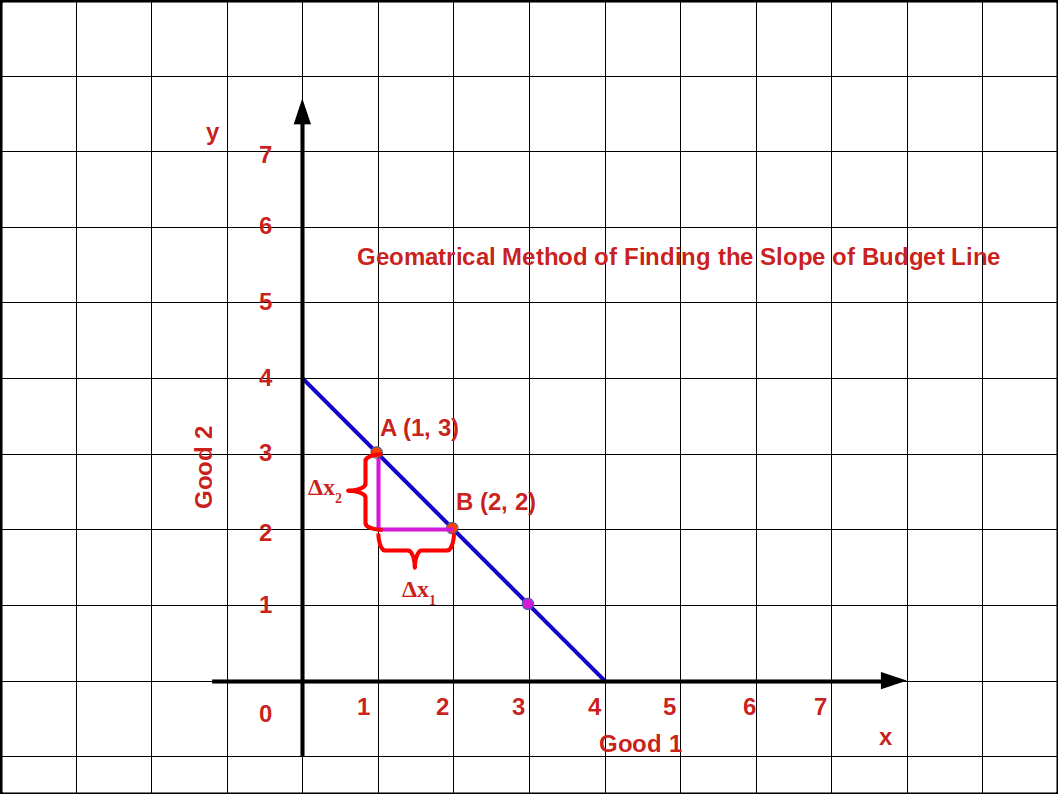
In the above given graph, when the consumer moves from bundle A to bundle B the decrease in good 2 is (Δx2) 1 unit. The increase in good 1 is (Δx1) 1 unit. Therefore, the slope of the budget line is \( {{{\frac {Δx_2}{Δx_1}}} = {{\frac {2 – 3}{2 – 1}}} = {{\frac {- 1}{1}}}} = -1\)
Changes in Budget Set
The consumption bundles available to a consumer depends on: (I) changes in the income of the consumer and (II) changes in the prices of goods. Therefore, any change in the prices of goods or income of the consumer may affect the budget set and budget line.
(I) Changes in the Income of the consumer
There are two types of changes in the income of the consumer. They are
- Increase in income and
- Decrease in income
a. Increase in income
When the income of the consumer increases, the consumer is able to buy more of two goods and the budget line shifts parallel outward. If his income increases from M to M’ the new budget line equation would be P1x1 + P2x2 = M’ and the vertical intercept of this budget line would be \( {\frac {M’}{P_2}} \) and horizontal intercept would be \( {\frac {M’}{P_1}} \). Budget lines with incomes M and M’ are given in below diagram.

Let us practice an example. Suppose the consumer’s income increases from ₹20 to ₹30 and the prices of good 1 and good 2 remain the same as ₹5. Then the new budget line equation would be 5x1 + 5x2 = 20. The vertical intercept and the horizontal intercept would be 6. When income increased from ₹20 to ₹30 vertical and horizontal intercepts shifted from 4 to 6, refer the below given graph.
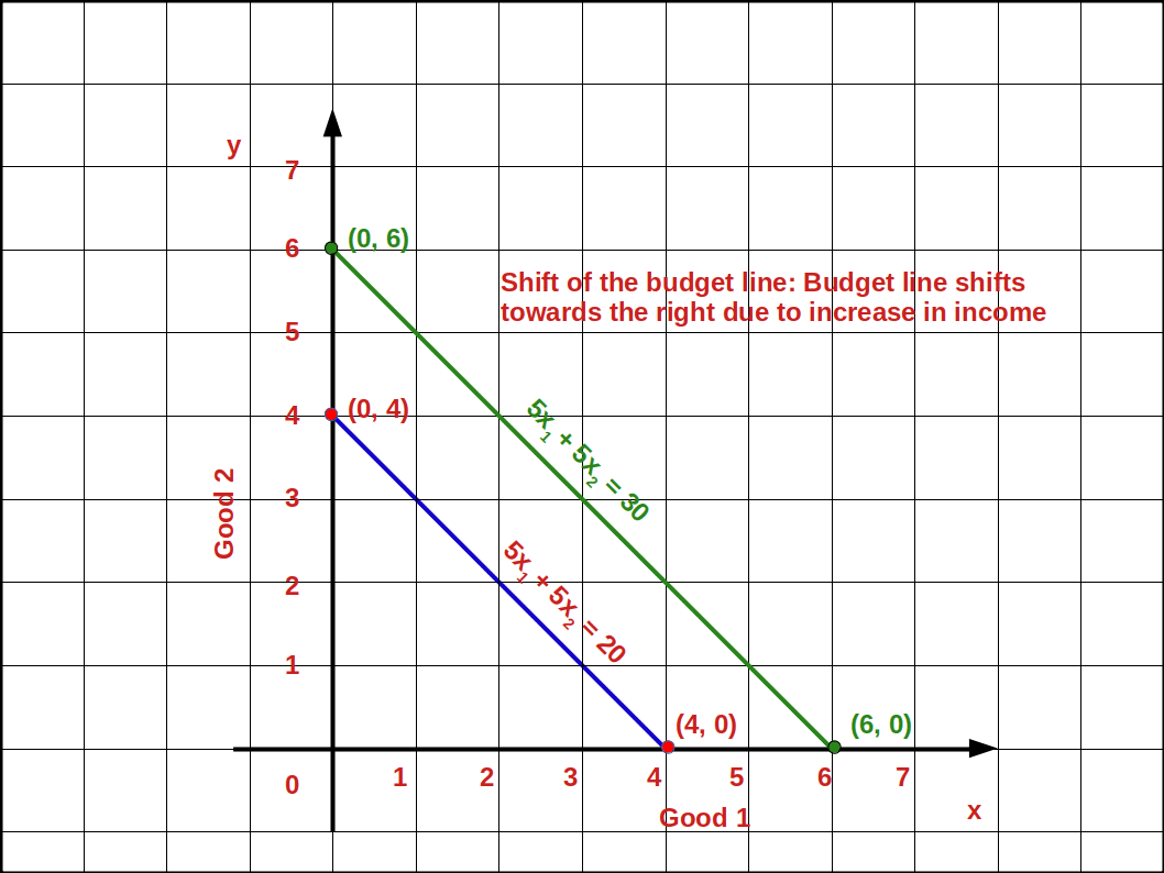
The budget line shifts from 51 +52 =20 to 51 +52 =30. Now the consumer can buy extra units of both goods. The slope of budget line \( {\frac {-P_1}{P_2}} \) remains -1.
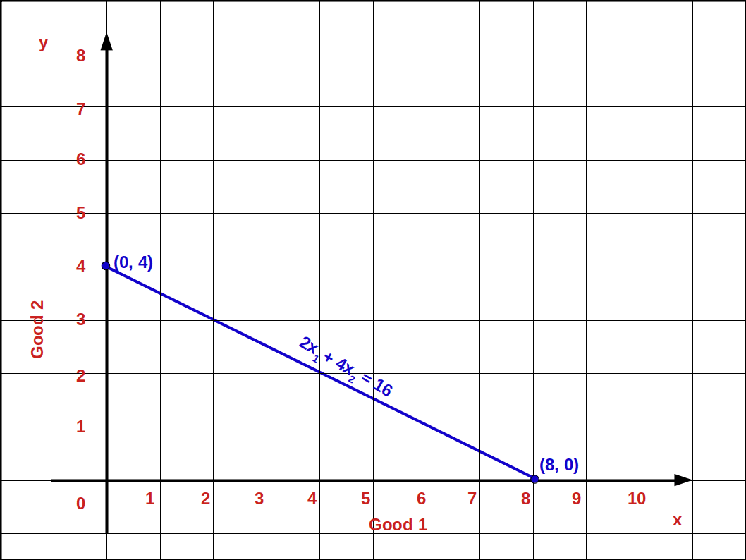
Let us practice an example. If P1 = 2, P2 = 4, M = 16.
- Write down the budget line equation.
- Find vertical intercept.
- Find horizontal intercept.
- What is the slope of the budget line ?
- Draw the budget line.
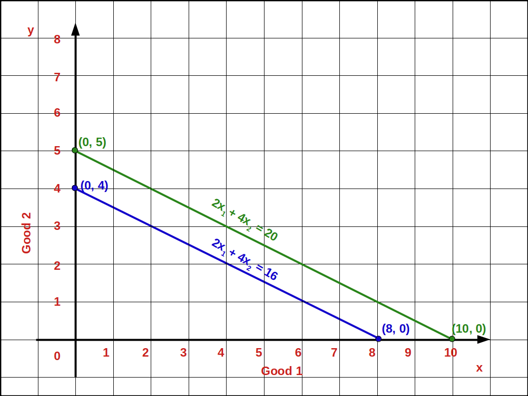
- M = 16 changes to M’ = 20. What happens to budget line? Draw the budget line.
- What is the slope of the new budget line ?
- 2x1 + 4x2 = 16
- Vertical intercept \( {{\frac {M}{P_2}} = {\frac {16}{4}}} =\,4 \) (0, 4)
- Horizontal intercept \( {{\frac {M}{P_1}} = {\frac {16}{2}}} =\,8 \) (8, 0)
- Slope \( {\frac {Δx_2}{Δx_1}} \)
= \( {\frac {-P_1}{P_2}} \)
= \( {\frac {-2}{4}} \)
= \( {\frac {-1}{2}} =\,-\,0.5 \)
-
- Vertical intercept \( {{\frac {M’}{P_2}} = {\frac {20}{4}}} =\,5 \) (0, 5)
- Horizontal intercept \( {{\frac {M’}{P_1}} = {\frac {20}{2}}} =\,10 \) (10, 0)
- \( -{\frac {P_1}{P_2}} \)
\( -{\frac{2}{4}} \)
\( {-\frac {1}{2}}=\,-\,0.5 \)
b. Decrease in income
When the consumer’s income decreases, he is not able to buy goods with the same amount. So the budget line shifts parallel leftward. When income decreases from M to M’1 (M’1 < M) the budget line shifts to the left. It is shown in the below Diagram.
| Table 2.2 Changes in Budget Line | ||
| Increase in Income | Decrease in Income | |
| M < M' | M > M’1 | |
|---|---|---|
| Budget line equation P1x1 + P2x2 = M’ | Budget line equation P1x1 + P2x2 = M’1 | |
| Vertical intercept moves up from \( \mathbf{\frac {M}{P_2}} \) to \( \mathbf{\frac {M’}{P_2}} \) | Vertical intercept moves down from \( \mathbf{\frac {M}{P_2}} \) to \( \mathbf{\frac {M’_1}{P_2}} \) | |
| Horizontal intercept moves up from \( \mathbf{\frac {M}{P_1}} \) to \( \mathbf{\frac {M’}{P_1}} \) | Horizontal intercept moves up from \( \mathbf{\frac {M}{P_1}} \) to \( \mathbf{\frac {M’_1}{P_1}} \) | |
| Consumer is able to purchase more quantities of both goods | Consumer is not able to purchase more quantities of both goods | |
| Budget line shift rightward | Budget line shift leftward | |
| Slope does not change | Slope does not change | |
Let us try to answer the below given problem.
The income of budget line 1 is ₹12 and that of the second one is ₹20. The slope of the first budget line equals the slope of the second budget line.
That is, \( -\,{\frac {P_1}{P_2}} \) = \( -\,{\frac {3}{4}} \) slope.
This is because there is no change in the prices of both the goods.
(II) Changes in Price
If price of goods changes without any change in consumer’s income, there will be changes in vertical – horizontal intercepts and slopes. There are two types of changes in the price of good 1. They are,
- Increase in price of good 1
- Decrease in price of good 1
- Increase in price of good 2
- Decrease in price of good 2
a. Increase in price of good 1
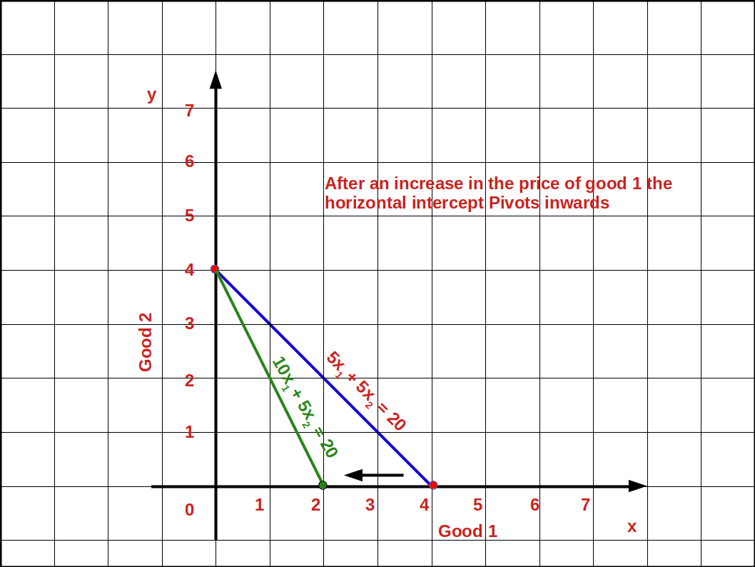
If the price of good 1 increases from P1 to P’1 and the price of good 2 and income of the consumer (M) remains unchanged, horizontal intercept of the budget line pivots inwards around the y-axis and the slope increases. Consumer is not able to buy good 1 with the same amount.
When price of good 1 increases from P1 to P’1, P’1x1 + P2x2 = M, is the equation of the budget line. Here, \( {\frac {M}{P_2}} \) is the vertical intercept and \( {\frac {M}{P_1}} \) is the horizontal intercept \( – {\frac {P_1}{P_2}} \) becomes the slope of the budget line. This is shown in the below given Diagram. Here we can see that due to an increase in price of good 1 horizontal intercept \( {\frac {M}{P_1}} \) moves inward to \( {\frac {M}{P’_1}} \). Moreover, there is no change in vertical intercept. It remains the same as \( {\frac {M}{P_2}} \).
Let us practice an example.
Price of good 1 increases from ₹5 to ₹10. Price of good 2 is ₹5 and the consumer’s income is ₹20. The new budget line would be 10x1 + 5x1 = 20.
Vertical intercept = 4 = \( \Bigl({\frac {M}{P_2}} = {\frac {20}{5}} = 4 \Bigr)\).
Horizontal intercept= 2 = \( \Bigl({\frac {M}{P’_1}} = {\frac {20}{10}} = 2 \Bigr)\).
The slope of the budget line is -2 because in order to get one unit of good 1, 2 units of good 2 have to be sacrificed. 5x1 + 5x2 = 20 is the old budget line and 10x1 + 5x1 = 20 is the new budget line as is shown in the below given graph. Here, we can see that the horizontal intercept of the new budget line has moved towards vertical axis.
b. Decrease in price of good 1
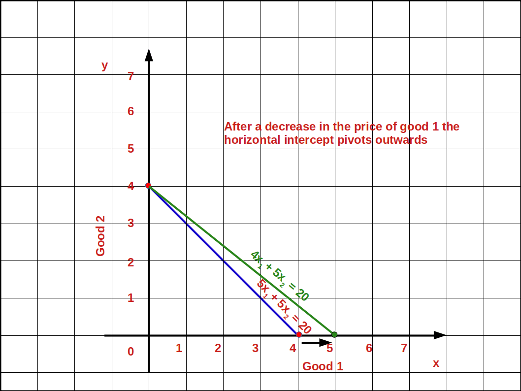
If the price of good 1 decreases from P1 to P’1 and the price of good 2 and income of the consumer (M) remain unchanged, horizontal intercept of the budget line pivots-outwards around the y-axis and the slope decreases. Consumer is able to buy more of good 1 and the budget line becomes less steep. This situation is shown in the below digram.
Let us practice an example.
In the budget line equation 5x1 + 5x2 = 20 if the price of good 1 decreases from ₹5 to ₹4 the vertical intercept of the new budget line, 4x1 + 5x2 = 20 will be 4 \( \Bigl({\frac {M}{P_2}} = {\frac {20}{5}} = 4 \Bigr)\).
The horizontal intercept will increase to 5 from 4 \( \Bigl({\frac {M}{P’_1}} = {\frac {20}{4}} = 5 \Bigr)\).
And the slope of the budget line changes from 1 to 0.8 \( \Bigl(-{\frac {P’_1}{P_2}} = -{\frac {4}{5}} = -0.8 \Bigr)\). Look at the budget line drawn in the below graph.
c. Increase in price of good 2
If the price of good 2 increases from P2 to P’2 and the price of good 1 and income of the consumer (M) remains unchanged, vertical intercept of the budget line pivots inwards around the x-axis and the slope decreases. Consumer is not able to buy good 2 with the same amount.
When price of good 2 increases from P2 to P’2, P1x1 + P’2x2 = M, is the equation of the budget line. Here, \( {\frac {M}{P_2}} \) is the vertical intercept and \( {\frac {M}{P_1}} \) is the horizontal intercept \( – {\frac {P_1}{P_2}} \) becomes the slope of the budget line. This is shown in the below given Diagram. Here we can see that due to an increase in price of good 2 horizontal intercept \( {\frac {M}{P_2}} \) moves inward to \( {\frac {M}{P’_2}} \). Moreover, there is no change in vertical intercept. It remains the same as \( {\frac {M}{P_1}} \).
d. Decrease in price of good 2
If the price of good 2 decreases from P2 to P’2 and the price of good 1 and income of the consumer (M) remain unchanged, vertical intercept of the budget line pivots-outwards around the x-axis and the slope increases. Consumer is able to buy more of good 2 and the budget line becomes more steep. This situation is shown in the below digram.
Preferences of the Consumer
The consumer chooses his consumption bundles from the budget set depending on his taste and preferences over the bundles. He compares the consumption bundles. And between any two consumption bundles, he prefers one bundle to the other or he is indifferent. The consumer ranks the bundles in the order of his preferences from the best to the least.
Consumption bundles as per budget set 5x1 + 5x2 ≤ 20 are ranked below in the order of preference.
| Table 2.3 | |
| Bundles | Ranking |
| (2, 2) | I |
|---|---|
| (1, 3), (3, 1) | II |
| (1, 2), (2, 1) | III |
| (1, 1) | IV |
| (0, 1), (0, 2), (0, 3), (0, 4), (1, 0), (2, 0), (3, 0), (4, 0) | V |
In the above Table most preferred bundle is (2, 2). Bundles (1, 3), (3, 1) are similar to the consumer. These bundles give the same level of satisfaction. Ranking or preferences will change according to personal preferences.
Monotonic Preference
Consumer’s preferences are said to be monotonic preferences, if between any two bundles, the consumer prefers the bundle which has more of at least one of the goods and no less of the other goods as compared to the other bundles. (x1, x2) and (y1, y2), are two bundles; if (x1, x2) has more of at least one of the goods and no less of the other goods as compared to (y1, y2), the consumer prefers (x1, x2) to (y1, y2). Simply monotonic preference means, the consumer prefers more amount of bundle than less amount of bundle and is called monotonic preference. In other words consumer prefers the superior bundle to the inferior bundle, when his preference is monotonic.
In Table 2.3, the consumer prefers (2, 2) to (2, 1). This is because in the bundle (2, 2) we have 1 unit more of good 2 as compared to the bundle (2, 1). If the consumer chooses the bundle (2, 1), his preference is not monotonic.
Substitution between Goods
Substitution between goods means the amount of good 2 that the consumer is willing to give up to get one unit of good 1. The rate at which one good is substituted for another is called rate of substitution.
It measures the consumers willingness to pay for good 1 in terms of good 2. The rate of substitution between good 2 and good 1 is given by the absolute value of Δx2 ÷ Δx1 where Δx2 represents change in good 2 and Δx1 represents change in good 1.
We can explain it with an example. Consider the bundles (2, 2) and (1, 3). Δx2 = (3 – 2) = 1 and Δx1 = (2 – 1) = 1. Therefore \( \vert{\frac {Δx_2}{Δx_1}} \vert\) = \( {\frac {1}{1}}\,=\,1\). Thus the rate of substitution between good 2 and good 1 is 1.
Diminishing Rate of Substitution
Let us assume that a consumer consumes two goods, good 1 and good 2. To obtain more units of good 1, he has to sacrifice some units of good 2. As the consumer consumes more and more units of good 1, the amount of good 2 sacrificed diminishes. This is known as Diminishing Rate of Substitution. The consumer’s preference of this kind is called convex preferences.
| Table 2.4 | |||||
| Good 1 | Good 2 | Δx1 | Δx2 | Rate of Substitution. \( \bigl( {\frac {Δx_2}{Δx_1}} \bigr) \) | |
|---|---|---|---|---|---|
| 10 | 20 | – | – | – | |
| 11 | 15 | 1 | 5 | 5 | |
| 12 | 11 | 1 | 4 | 4 | |
| 13 | 8 | 1 | 3 | 3 | |
| 14 | 6 | 1 | 2 | 2 | |
| 15 | 5 | 1 | 1 | 1 | |
Look at the above table. All are indifferent bundles. All these bundles give same level of satisfaction. As the consumer substitutes more and more units of good 1 for good 2 the absolute value of rate of substitution declines from 5 to 1.
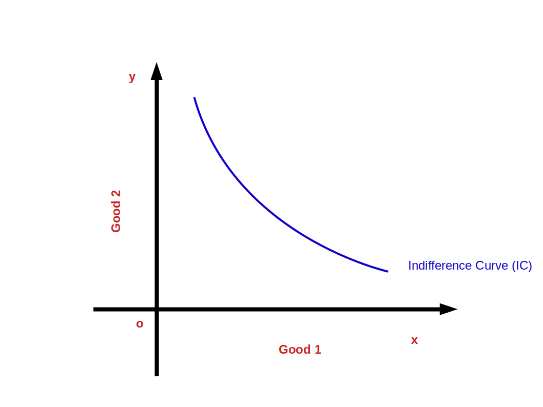
Indifference Curve Indifference Curve is defined as the locus of points of combinations of two goods, good 1 and good 2, which gives the consumer the same level of satisfaction. It is the graph showing the bundles that give the consumer the same level of satisfaction. This is shown in below given diagram.
Points on, above and below the indifference curve
 In the above given Diagram, A and B are two points on the indifference curve. The consumption bundles (X1, Y2) and (X2, Y1) give him the same level of satisfaction. The bundles A and B are known as efficient bundles. Any bundle outside the indifference curve, e.g., the bundle at point D is the preferred bundle. But any bundle below the indifference curve is an inferior bundle. For example, C is an inferior bundle.
The Rate of Substitution and the Slope of Indifference Curve The slope of indifference curve is equal to the rate of substitution. When the amount of good 1 increases by one unit, the amount of good 2 decreases by same unit. The rate of substitution or Marginal Rate of Substitution (MRS) is the absolute value of the ratio of the good sacrificed and the good obtained. This is the same as the slope of the indifference curve. This is shown in the below Diagram.

Slope of the indifference curve = Rate of Substitution = Marginal Rate of substitution = \(\mathbf{\frac{ΔX_2}{ΔX_1}} \)
As the indifference curve slopes down,
\( \mathbf{{MRS_{x1x2}}\,=\, -\,{\frac{ΔX_2}{ΔX_1}}} \)
Diminishing Marginal Rate of Substitution (DMRS) As the consumer moves along the indifference curve from left to right, the amount of good 1 increases and the amount of good 2 decreases. The marginal rate of substitution between good 1 and good 2 goes on decreasing. This is known as Diminishing Marginal Rate of Substitution (DMRS).
| Table 2.5 | |||
| Bundles | Good 2 (x2) | Good 1 (x1) | MRSx1x2 = \( \bigl( {\frac {Δx_2}{Δx_1}} \bigr) \) |
|---|---|---|---|
| a | 11 | 1 | – |
| b | 7 | 2 | 1:4 |
| c | 4 | 3 | 1:3 |
| d | 2 | 4 | 1:2 |
| e | 1 | 5 | 1:1 |
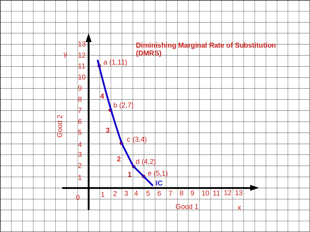
In the Table 2.5 when the consumer moves from bundle a to b, b to c, c to d and d to e, MRS goes on decreasing. MRSx1x2 4, 3, 2, 1. This is shown in the above Graph.
Indifference Map A collection of indifference curves is known as Indifference Map. The below given Diagram shows an indifference map.
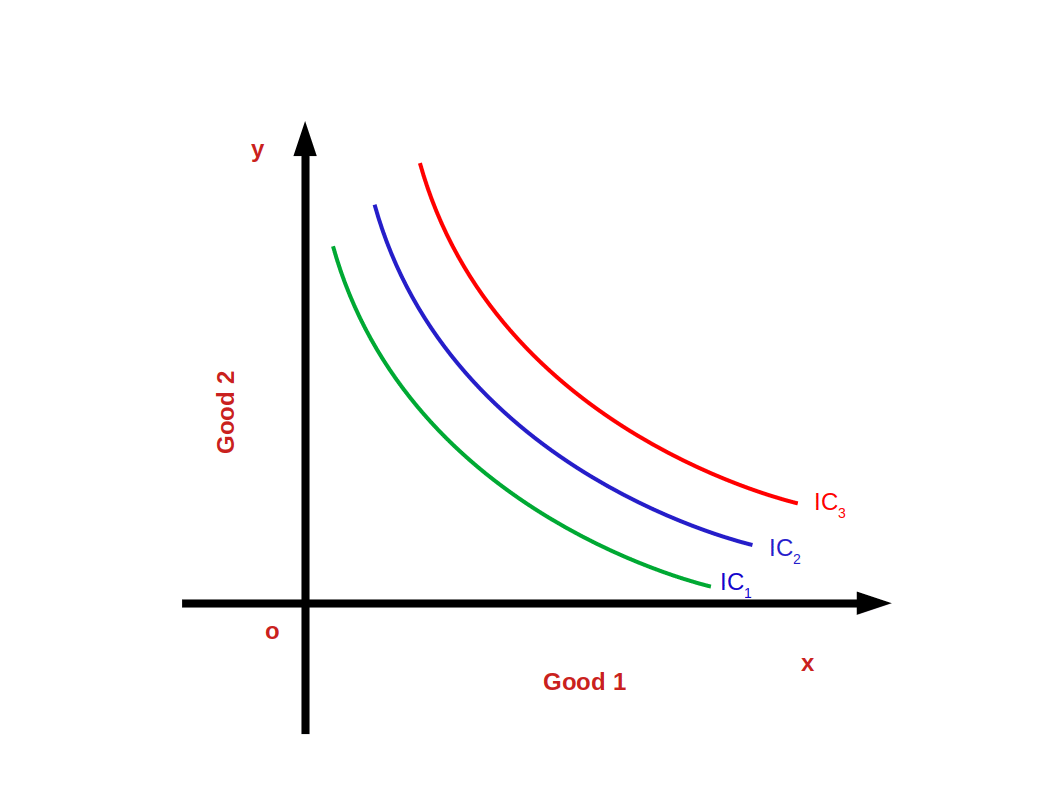
The satisfaction derived from the bundles on the indifference curves IC1, IC2 and IC3 are different. IC2 gives more satisfaction than IC1. IC3 gives much more satisfaction than IC2.
$$ \mathbf{IC_3 > IC_2 > IC_1} $$
Properties (Features) of Indifference Curves
- Indifference curves slope down wards from left to right.
- Indifference curves are convex to the origin. (Because of diminishing marginal rate of substitution).
- Higher indifference curves represent higher levels of satisfaction.
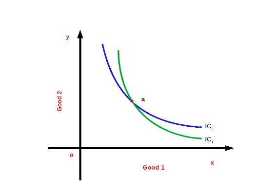
- Indifference curves do not intersect each other. This can be proved with the help of given below diagram. As per the diagram, point a which lies on IC1 and IC2 gives the same level of satisfaction. This is not true. IC2 represents higher level of satisfaction than IC1.

Utility The power of a commodity to satisfy human wants is called utility.
The numbers given to the bundles are called utilities of the bundles. The representation of preferences in terms of utility numbers is called a utility function or a utility representation. The most preferred bundle gets higher utility numbers and the least preferred bundle gets lower utility numbers. Indifferent bundles may have same utility numbers. Table 2.6 gives the utility representation.
| Table 2.6 | |||
| Bundles of two goods | Utility representation | ||
| (2, 2) | 40 units | ||
|---|---|---|---|
| (1, 3), (3, 1), 0, 4), (4, 0) | 35 units | ||
| (1, 2), (2, 1), (0, 3), (3; 0) | 28 units | ||
| (0, 2), (2, 0), (1, 1) | 20 units | ||
| (0, 0), (0, 1), (1, 0) | 10 units | ||
The utility number assigned to the bundle (2, 2) is 40. The utility number assigned to the bundles (1, 3), (3, 0), (0, 4) and (4, 0) is 35. The utility number assigned to the bundles (1, 2), (2, 1), (0, 3) and (3, 0) is 28 and so on. The bundle (2, 2) has the highest utility number because it is the most preferred bundle. On the other hand, the bundles (0, 0) (0, 1) and (1, 0) have lower utility number 10.
Consumer’s Equilibrium
(Consumer Optimum) Consumer’s equilibrium can be defined as the position of maximum satisfaction.
According to indifference curve approach, a consumer attains equilibrium at the point where budget line is tangent to indifference curve or MRS equals price ratio or slope of indifference curve (MRS) is equal to slope of budget line, i.e., price ratio \( \bigl( {\frac {- P_1}{P_2}} \bigr) \)
Look at the above given Diagram. BL is the budget line and IC1, IC2, and IC3, are different indifference curves. At point E the slope of the budget line and the slope of IC, become equal \( \bigl( {\frac {Δx_2}{Δx_1}}\, = \, MRS_{x1x2}\, = \, {\frac {- P_1}{P_2}} \bigr) \). At point E, the consumer is at equilibrium. As he chooses the bundle (x1*, x2*) he gets maximum satisfaction.
The consumption bundles on IC1 give less satisfaction than the bundles on the indifference curve IC2. The bundles on IC3 give more satisfaction than the bundles on indifference curve IC2. The consumer cannot get the bundles on IC3 because all the bundles on IC3 are beyond his budget line. Therefore, the bundle (x1*, x2*) gives him the maximum Satisfaction.
Demand A consumer’s desire to buy a good is usually considered as demand. But in economics mere desire does not become demand. The consumer should have the ability and willingness to buy along with his desire for a good. Therefore, Demand-is desire backed by willingness to pay and ability to pay.
Demand for a Commodity Demand for a commodity is the quantity of a commodity that a consumer is willing to buy in a given period of time at a given price.
The quantity of the good a consumer decides to buy depends on the price of the good, the prices of other goods, the income of the consumer and the taste and preferences of the consumer. The demand is a multivariate relationship. It is determined by various factors simultaneously. When changes occur in the factors or determinants change also takes place in the quantity of the good he decides to buy.
Individual Demand Individual demand can be defined as the quantity of a commodity that an individual consumer is willing to buy from the market in a given period of time at a given price.
Household Demand Household demand can be defined as the quantity of a commodity that a household is willing to buy from the market in a given period of time at a given price.
Demand Function The functional relationship between demand and the determinants of demand is called Demand Function, i.e., the relationship between demand (q) and its determinants such as price of the commodity (P), Income of the consumer (M), Prices of related commodities (Pr) and Taste and preference of the consumer (T).
$$ \mathbf{Algebraically, q = f(P, Pr, M, T)} $$
The price, P is the most important factor among the determinants of demand. Therefore, the consumer’s demand for a commodity can be written as the function of price.
$$ \mathbf{q \,=\, d(P)} $$
Law of Demand The consumer’s demand for a commodity and its price have a negative or inverse relationship. Other things remaining unchanged, the inverse relationship between demand and price of the commodity is called law of demand. That is, as the price of the commodity falls the quantity demanded rises and as the price rises quantity demanded falls, other things remaining unchanged. The Law of Demand is based on the assumption that the consumer’s income, prices of related commodities, tastes and preferences of the consumer are constant.
Demand Curve The graph which shows the inverse relationship between demandand price is called Demand Curve. In other words, the graphical representation of the demand function is called the demand curve. Below Diagram shows a demand curve.
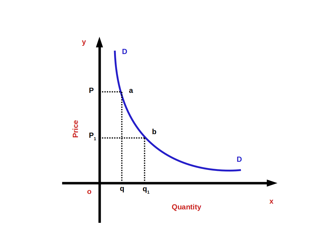
Quantity is represented along x-axis and price is represented along y-axis. DD is demand curve. This curve shows the inverse relationship between price and demand. When price rises from OP1 to OP quantity demanded falls from Oq1 to Oq. When price falls from OP to OP1 quantity demanded rises from Oq to Oq1. So the curve DD shows the inverse relationship between price and demand. That is why the demand curve is sloping downward from left top to right bottom. The slope of demand curve is negative.
Why does demand rise when price falls? Substitution effect and income effect are the two main reasons for the inverse relationship between price and quantity demanded. The sum of substitution effect and income effect is price effect.
Price effect:
Change in demand caused by change in price is called price effect. Price effect can be divided into two: substitution effect and income effect.
Substitution effect:
Substitution effect considers two commodities When there is a fall in the price of one of them; there is a change in relative price. As a result more of the cheaper good is demanded instead of the good with unchanged price. The cheaper good is substituted in the place of the costlier good.
Income effect:
Income effect is the change in the demand of a commodity due to the change in real income of the-consumer. When price of a commodity goes down, purchasing power increases. This is an increase in real income. As a result, the consumer demands more of it.
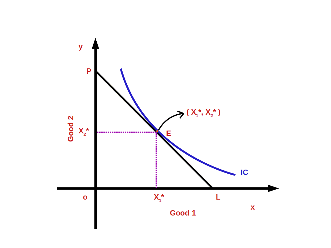
Look at the above diagram. Here on the budget line PL at point E the consumer is in equilibrium State. The budget line PL touches the indifference curve IC at point E.
The Consumer’s equilibrium bundle is (x1*, x2*). The cost of this bundle is P1x1* + P2x2* = M, When the price of one commodity falls two changes take place:
Suppose the price of good 1 falls
- The price of good 1 falls when compared good 2. That is relative price falls. This makes the consumer capable of buying more units of the less expensive good.
- As his purchasing power has increased, the consumer’s real income increases. This enables the consumer to buy the same quantity of goods before price fall for a lesser price.
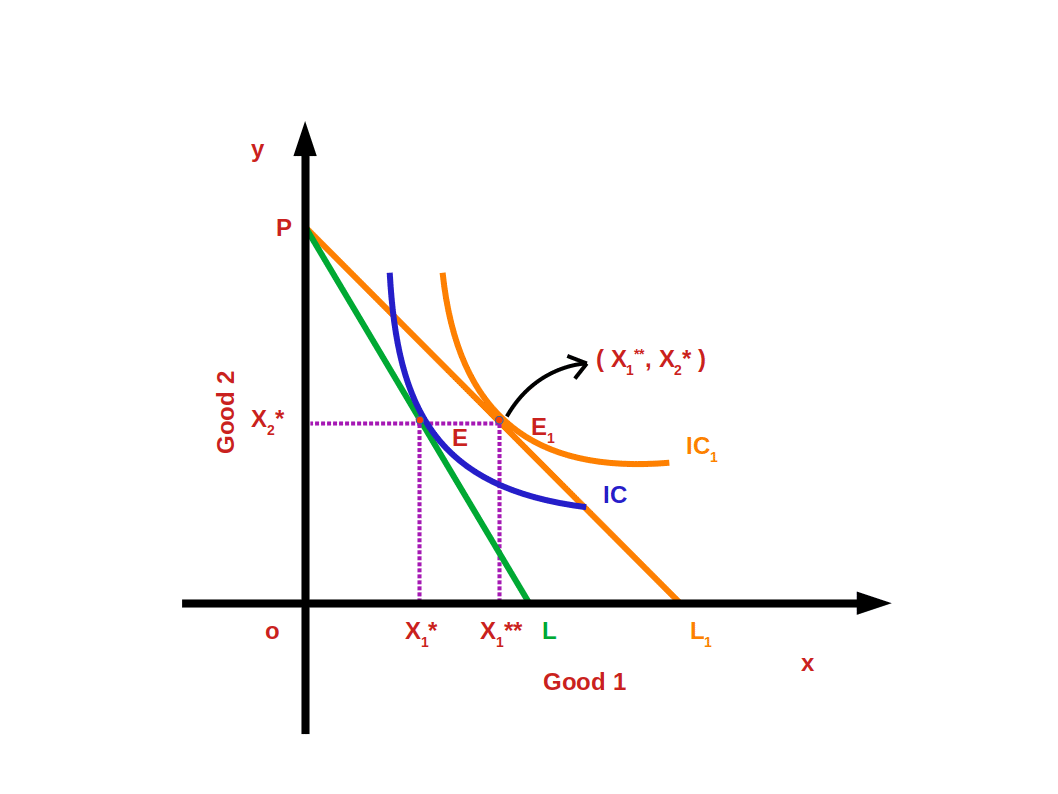
Look at the above diagram. The price of good 1 has fallen. As a result the budget line PL has changed to PL1. The indifference curve IC1 touches the budget line PL1, at point E1. At point E1 the consumer accepts the bundle (x1**, x2*) and he is in equilibrium stage. Bundle E (x1*, x2*) changes to the new bundle E1 (x1**, x2*). This change from E to the new bundle E1 (x1**, x2*) is called price effect.
As a result of fall in price of good 1 the measure of demand for good 1 increases from x1* to x1** . The change in the demand of good due to change in price is called price effect. Price effect is the combination of substitution effect and income effect. Price effect can be divided into substitution effect and income effect. To separate substitution effect and income effect we have to remove the gain in real income due to price fall. That is to say, to separate price effect into substitution effect and income effect we have to bring about a change in the expense that would enable him to select the bundle before price change.
Suppose the price of good 1 changes from P1 to ΔP1
Now the new price of good 1 is P1 – ΔP1. The price of good 2 remains unchanged as P2.
The price of the bundle ( x1*, x2* ) would be
= ( P1 – ΔP1)x1* + P2x2*
= P1x1* – ΔP1x1* + P2x2*
= P1x1* + P2x2* – ΔP1x1*
= M – ΔP1x1* ( P1x1* + P2x2* = M )
So there is a decrease in the income of the consumer ΔP1x1*. The difference in expense would be ΔP1x1*.
i.e. change in expenses before and after change in price would be ΔP1x1*.
Price fall of good 1 causes gain in income. To counter this gain in income, expenses are to be changed. Change in expense in (ΔP1x1*.). This is to be subtracted from the consumer’s income.
$$ {i.e,\, (M-ΔP_1{x_1^*} )} $$
In the below diagram the budget line changes to P’L’. The budget line P’L’ passes towards the left through the bundle E and parallel to the budgetline PL1.
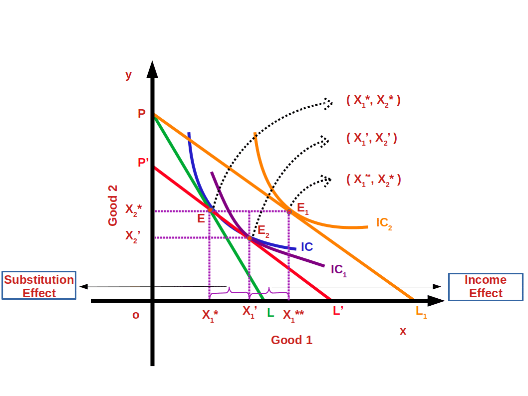
Now the consumer has adjusted his income equal to his previous purchasing power. The change from point E to point E2 is called substitution effect. Demand for good 2 is decreased from x2* to x2‘ at point E2. Thus the means of good 1 increase from x1* to x1‘ . In the place of bundle (x1*, x2*) bundle (x1‘, x2‘ ) is substituted. More of the cheap good is substituted in the place of goods with unchanged price. This is known as Substitution Effect.
The change from point E2 to point E1 is called Income Effect. He changes from the bundle ( x1‘, x2‘ ) to the bundle ( x1**, x2* ). When there is a change in the price of good 1 there is a corresponding change in the purchasing power. This causes changes in measure of demand, and is called income effect.
Total effect is the change from E to E1 . It is the sum of substitution effect and income effect.
$$ {i.e,\,PE \,=\, SE \, + \, IE} $$
Therefore there exists an inverse relationship. These two affects, the amount of demand and its price.
Let us explain these effects using numerical data. Suppose a consumer’s income is ₹30.
Price of good 1 = ₹10
Price of good 2 = ₹5
The consumer’s most preferred bundle is (2, 2). In the below graph, the most preferred bundle (2, 2) is marked in the budget line 10x1 + 5x2 = 30.
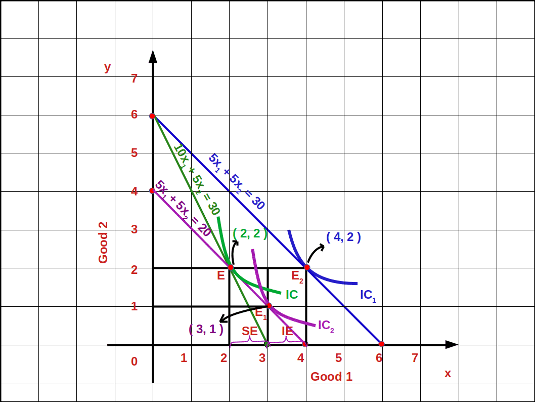
Now let us suppose that the price of good 1 falls from ₹10 to ₹5. The relative price also comes down. Now the budget line is 5x1 + 5x2 = 30 and the consumer’s most preferred bundle is (4, 2).
The change from bundle (2, 2) to the bundle (4, 2) is called price effect. That is, as the price of good 1 decreased the consumer can buy 4 units of it instead of 2 units, More than that, because of price fall, the consumer can buy the first bundle (2, 2) for ₹20. This is income effect.
₹5×2 + ₹5×2 = ₹10 + ₹10 = ₹20
If the consumer’s income comes down by ₹10 (₹30 – ₹20 = ₹10) he can manage to buy the bundle (2, 2). Then the budget line would become 5x1 +5x2 = 20. This budget line moves towards the left and goes parallel to the budget line. 5x1 +5x2 = 30. Now the consumer gets an additional income of ₹10. With this money he can buy more units of the good, if he wants. If he wants to buy more of good 1 he will be able to buy 5x1 = 10.
\( x_1\,=\,{\frac{10}{5}}\,=\,2 \) (two units).
If he wants to buy more of good 2 he can buy 5x2 = 10.
\( x_2\,=\,{\frac{10}{5}}\,=\,2 \) (two units).
Or he can buy one unit extra each of good 1 and good 2.
So, when price falls due to substitution effect and income effect, its demand increases. That’s why the demand curve has a negative slope.
When measure of good 1 increases from 2 units to 4 units it is price effect. When the measure of good 1 increases from unit 2 to unit 3 it is substitution effect.
When the measure of good 1 increases from 3 to 4 units it is income effect.
Linear Demand The relation between demand and price can be linear or non linear. A linear demand curve can be algebraically written as
$$ {q\,=\,a\,-\,bP\,;\,0≤P≤ {\frac{a}{b}}} $$
$$ {=\,0\,;\,P > {\frac{a}{b}}} $$
In this linear demand equation
a is vertical intercept
-b is the slope of the demand curve
P is price of good
q is quantity demanded
Moreover,
$$ {If\, price\, =\, 0} $$
$$ {demand \,will \,be \,=\,a} $$
$$ {If\, price\, is \,=\,{\frac{a}{b}}}$$
$$ {demand \,will \,be \,=\,0} $$
Look at the below diagram.
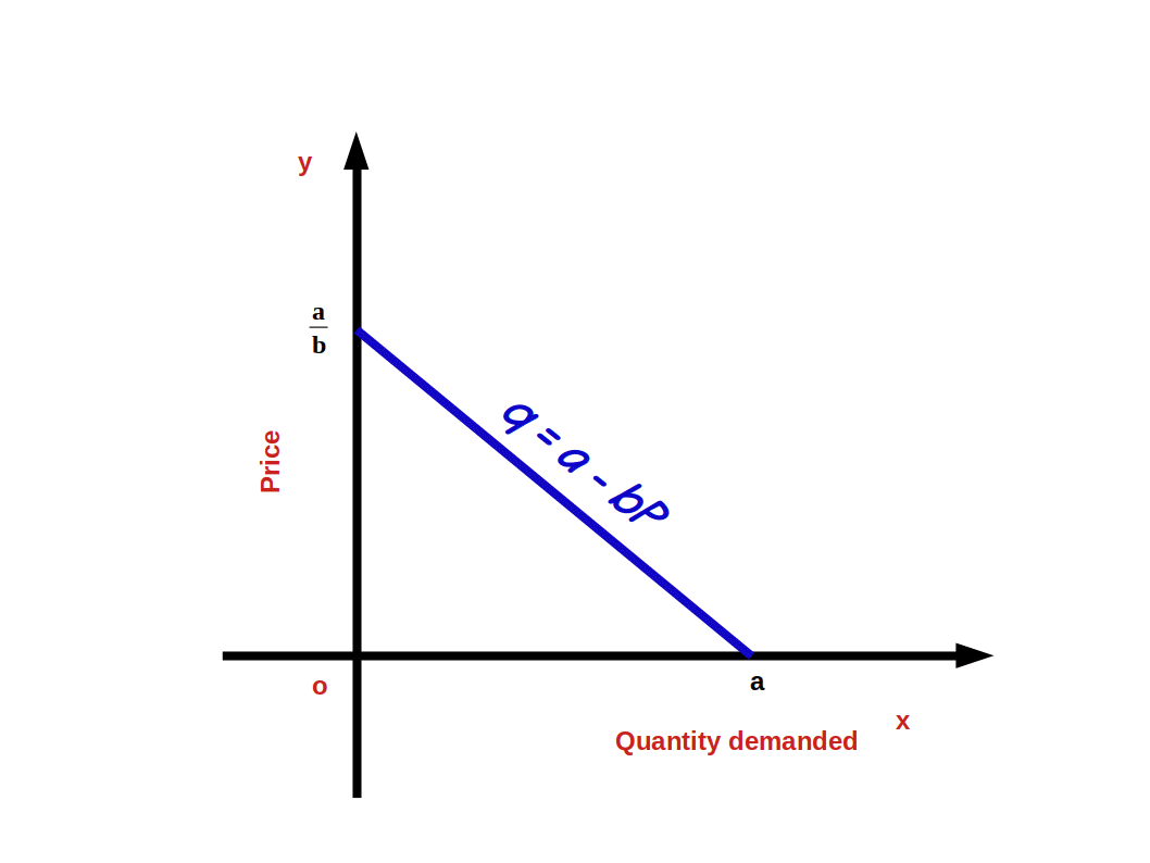
Linear demand curve is shown in the above given diagram. The slope of the demand curve indicates the rate of change in demand according to change in price. That means, whenever there is a change of one unit in price, demand changes by —b unit. Since b is negative the relation between demand and price will be inverse. If price rises by 1 unit, demand will fall by —b unit. Since b is negative the relation between demand and price will be inverse. Price increase by one unit brings down demand by b unit.
$$ {Demand \,curve \,slope\,{\frac{Δq}{ΔP}}\,=\,-\,b}$$
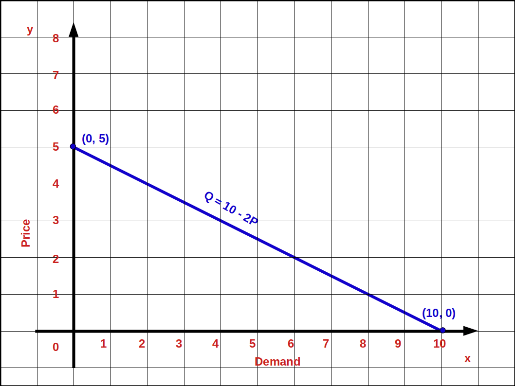
In the law of demand equation we can give values to a and b and the demand curve. Suppose
a = 10
b = 2
Then we get the demand equation
$$ {\,q \,=\,10\,-\,2P} $$
Here 0 ≤ P ≤ 5
If P > 5 demand will be 0
When P = 0, q = 10
i.e. q= 10 – 2 x 0 = 10 – 0 = 10
This is the horizontal intersect. If demand is 0 price would be 5.
0 = 10 – 2P (q = 0)
2P = 10
P = \({\frac{10}{2}} \) = 5, This is Vertical intercept.
Below given graph gives linear demand curve.
Using the law of demand equation q = 10 – 2P, we can find the different values of demand when price changes from 0 to 5, This is given in table 2.7.
| Table 2.7 | |||
| Price (P) | Demand (q) | Method of calculation. q = 10 – 2P | |
|---|---|---|---|
| 0 | 10 | q = 10 – 2 × 0 = 10 – 0 = 10 | |
| 1 | 8 | q = 10 – 2 × 1 = 10 – 2 = 8 | |
| 2 | 6 | q = 10 – 2 × 2 = 10 – 4 = 6 | |
| 3 | 4 | q = 10 – 2 × 3 = 10 – 6 = 4 | |
| 4 | 2 | q = 10 – 2 × 4 = 10 – 8 = 2 | |
| 5 | 0 | q = 10 – 2 × 5 = 10 – 10 = 0 | |
The table showing the relations between a consumer’s demand and price is called individual demand schedule.
Factors determining demand for a commodity or determinants of demand.
As per conventional principle of demand, demand for a commodity is determined mainly by four factors – price, income, price of other commodities and the consumer’s tastes and preferences. We shall now see how these factors affect demand.
Price of a commodity or own Price
The most important factor that determines demand for a commodity is its price. There is an inverse relation between the price and demand of a commodity. That is, when price increases demand decreases; when price decreases demand increases. This is very clear from the law of demand.Income of the consumer
Another’ factor that determines demand is the consumer’s income. The relation between income and demand depends on the nature of goods. Based on income we can divide goods into normal goods and inferior goods.- Normal goods: When the consumer’s income increases demand for the goods increases; when his income decreases demand also decreases. Such goods are called normal goods.
- Inferior goods: When the consumer’s income increases, demand decreases; when his income decreases demand increases. These goods are called inferior goods. The relation between Demand for such goods and the consumer’s income is inverse.
Prices of other related goods
The price of other related goods is another factor that determines the demand for a commodity. On the basis of the relation between its price and demand goods can be classified under two heads-- Substitute goods: Goods that are used as substitutes to satisfy a need are called substitute goods.
- Complementary goods: When more than one good are required to satisfy a want, such goods are called complementary goods.
Taste and preferences
Another factor that determine price is the taste and preferences. When the taste of a consumer for a particular good increases, demand for that good also increases, when his taste for such goods decreases demand for that good also decreases.
Goods like TV, computer, good clothes etc. are normal goods for one person; to another person, these things may not be normal goods, Relation between the consumer’s income and his demand for normal goods is positive. i.e.,consumer’s income and demand for mormal goods move in the same direction.
Kerosene stove is inferior to gas stove. Bus travel is inferior to travel by car. Cheap food grains is inferior to rice.
(a) Substitute goods
(b) Complementary goods.
Coffee and tea, bus and train, car and jeep, shoes and slippers are examples for substitute goods. Relation between price of substitute goods and demand is positive. On two substitute goods the price of one will change in the same direction as the demand for the other. When price of tea increases, demand for coffee increases; when price of tea decreases demand for coffee also comes down.
Pen and ink, car and petrol / diesel, lock and key and shoes and socks are complementary goods. The relation between price and demand of comple- mentary goods is inverse. They move in opposite directions. That is, when the price of one complementary good increases the demand for the other decreases. When price decreases demand increases.
Changes in Demand Changes in demand can be generally divided into two:
1. Movement along the demand curve
2. Shift of the demand curve
Movement along the demand curve
Change in demand due to change in price is called movement along the demand curve. Change occurs in the demand ‘curve because of the change in the price of the commodity. No change takes place in non-price factors like the consumer’s income. Price of other related goods, consumers tastes and preferences. Change along the demand curve can be of two types-Shift of Demand Curve
Change in the demand for commodity caused by changes in non-price factors is called shift of Demand Curve. Changes in factors other than price cause shift in the demand curve, For example, change in income. Shift of demand curve can be of two types:
(a) Expansion of demand
(b) Contraction of demand
Expansion of demand:
Downward movement along the demand curve due to fall in price is called expansion of demand. Increase in demand due to price decrease is called expansion of demand.
Look at the below given diagram. When the price of the commodity goes down from P to P1 demand increases from q to q1. In the demand curve, DD, there is a change from point ‘a’ to point ‘b’. This change from a to b is expansion of demand.

Contraction of Demand:
Upward movement along the demand curve due to price rise is called contraction of demand. In other words, when price of a commodity increases due to a fall in demand we call it contraction of demand.
In the below diagram, the price of a commodity increases from P1 to P. And demand for the commodity decreased from q1 to q. On the demand curve DD from point there is a shift from point b to point a. This change from point b to point a is called contraction of demand.
(a) increase in demand
(b) decrease in demand
Increase in demand:
Rightward or upward shift of the demand curve due to favourable changes in non-price factors is called increase in demand. In other words, when more quantity is demanded at a given price or the same price is known as increase in demand. Look at the below given diagram. There DD is the first demand curve. There is a demand for good Og at price OP. As a result of favourable changes in non-price factors DD changes to the new demand curve D1 D1 and goes towards the right. Then demand increases from Oq to Oq1 . The price continues the same OP. The change towards the right of demand curve DD to D1 D1 is called demand increase.
Decrease in demand:
On account of unfavourable changes in non-price factors the demand curve changes towards the left or downward. This change of the demand curve is called decrease in demand. That means, when less quantity is demanded at the given price or the same price, we have decrease in demand. In the below given diagram DD is the first demand curve. At price OP, Oq goods are demanded . On account of unfavourable changes in non price factors the demand curve DD changed towards the left to the new demand curve D1D 1. Then demand decreases from Oq to Oq1. But the price OP remains unchanged . Decrease in demand is then , the change towards the left of demand curve DD to D1D1.
Market Demand Market Demand is the quantity of a commodity that all consumers in a market are willing to buy at different prices at a fixed or given time. This is the total of individual demands. This is done by adding up horizontally all the individual demand tables. Look at the table 2.8. It icludes two individual demand and market demnad.
| Table 2.8 Market Demand | |||||
|---|---|---|---|---|---|
| Indiidual A | Individual B | Market Demand (Demand A + Demand B) |
|||
| Price | Demand | Price | Demand | Price | Demand |
| 10 | 5 | 10 | 7 | 10 | 12 |
| 20 | 4 | 20 | 6 | 20 | 10 |
| 30 | 3 | 30 | 5 | 30 | 8 |
| 40 | 2 | 40 | 4 | 40 | 6 |
The total of these two individual demand tables Individual A and Individual B is given in Market Demand column.
Market Demand Curve Market Demand Curve is formed from individual demand curves. By adding the demand curves of all individuals in a market we get the market demand curve. The total of all the demand curves of all individuals in a market is the market demand curve.
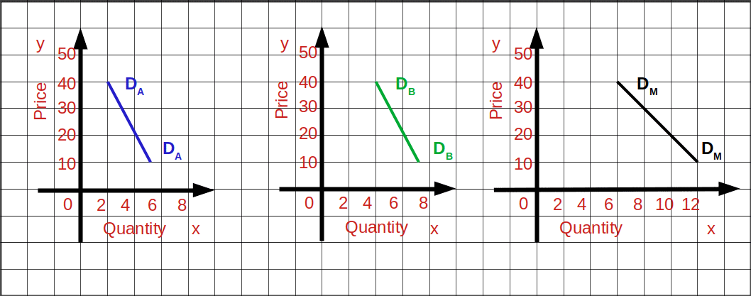
DA and DB are the individual demand curves of individual A and individual B. MD is the market demand curve.
Adding up of Two Linear Demand Curves Given below are the demand equations of two consumers.
$$ {\,d_1(P) \,=\,10\,-\,P}\, ; \,{0\,≤\,P\,≤\,10}$$
$$ {\,= \,0\,;\,P\,>\,0} $$
$$ {\,d_2(P) \,=\,15\,-\,P}\, ; \,{0\,≤\,P\,≤\,15}$$
$$ {\,= \,0\,;\,P\,>\,0} $$
If the price of the commodity is ₹10 or more the first consumer’s demand would be O. Similarly, if the price of the second commodity is ₹15 or more the second consumer’s demand would be O. To find the market demand we have to add these two individual demand equations.
Market demand equation (d(M))
$$ {\,d_1(P) \,+\,d_2(P) \,=\,10\,-\,P\,+ \,15\,-\,P}$$
$$ {d_(m)\, = 25 \,-\,2P\,;\,0\,≤\,P\,≤\,\frac{25}{2}} $$
$$ {0\, = 25 \,;\,P\,>\,\frac{25}{2}} $$
Price Elasticity of Demand
In Economics elasticity in very important. It was Alfred Marshal who first used the concept of elasticity in Economics. Price Elasticity can determine the amount of change in demand brought about by price changes. The word elasticity means responsiveness. Price elasticity of demand may be defined as the degree of responsiveness of quantity demanded of a commodity in response to change in its
price.
Price elasticity of demand is determined by the degree of change in quantity demanded in response to change in its price. On dividing the percentage of the change in demand by the percentage of change in price we get price elasticity.
Degree of Price Elasticity Elasticity will be different for different commodities. On the basis of rate of change in the quantity demanded, elasticity can be divided into five:
1. Elastic Demand (e > 1)
If the percentage of change of demand is greater than the percentage of change in price, it is called elastic demand. For example, when price changes by 10% demand increases by 30%. When elasticity of demand is high, the absolute value of elasticity will be more than one.
i.e. (│e│ > 1 or e < -1).
In the above example,
\( \vert e \vert \,=\,{\frac{30%}{10%}}\,=\,3. \)
Then Demand curve will be more flat as shown in the below diagram. Or the slope will be less.
2. Inelastic Demand (e < 1)
If the percentage change in demand is less than the percentage change in price, it is called inelastic demand or less elastic demand, For example, when percentage change in Price is 20% and change in demand is only 10%. In inelastic demand the absolute value of elasticity would be less than one.
i.e. (│e│ < 1 or e > -1)
In the above example,
\( \vert e \vert \,=\,{\frac{10%}{20%}}\,=\,0.5. \)
In this case demand curve would be less flat or more steep as shown in the blow Diagram.
3. Unitary Elastic Demand (e = 1)
If the percentage change in demand and percentage change in price are equal, it is called unitary elastic demand. For example, when there is 10% change in price it results in 10% change in demand.
Under unitary elastic demand, the absolute value of elasticity will be one.
i.e. (│e│ = 1 or e = -1)
In the above example,
\( \vert e \vert \,=\,{\frac{10%}{10%}}\,=\,1. \)
Then the demand curve would have a moderate slope as shown in the below given diagram.
4. Perfectly Elastic Demand (e = ∞)
When a small change in price leads to infinite change in demand, we have perfectly elastic demand. In such cases, the absolute value of elasticity would be infinite or unlimited.
i.e. (│e│ = ∞ or e = -∞)
and the demand curve would be parallel to x-axis or horizontal as shown in the below Diagram. The slope of demand curve would be 0.

5. Perfectly Inelastic Demand (e = 0)
Perfectly inelastic demand is a situation in which, whatever may be the changes in price, quantity demanded is un-affected. In this case the value of elasticity would be 0. Then demand curve would be
vertical to x – axis as shown in the below Diagram.
i.e. (│e│ = 0 or e = 0)
Among the five degrees of elasticity of demand, perfectly elastic demand and perfectly inelastic demand are rare in practical life.
Methods of measuring Price Elasticity of Demand
Price elasticity is measured in three different ways:
(1) Percentage method
(2) Measurement of elasticity along a linear demand curve
(3) Expenditure method
(1) Percentage method
Under percentage method price elasticity of demand is measured by dividing the percentage change in quantity demanded by the percentage change in price.
Price elsticity of demand = $$ \mathbf {{\frac{Percentage\,change\,in\,quantity\,demanded}{Percentage\,change\,in\,price}}} $$ $$ \mathbf {e \,=\,{\frac{{\frac{Change\, in\, quantity}{Initial\, quantity}}× 100}{{\frac{Change\, in\, price}{Initial\, price}}× 100}}} $$If P = initial price, q = initial quantity demanded, ΔP.= change in price and Δq = change in quantity demanded then,
$$ \mathbf {e \,=\,{\frac{{\frac{Δq}{q}}× 100}{{\frac{ΔP}{P}}× 100}}} $$
$$ \mathbf {e \,=\,{{{{\frac{Δq}{q}}}}÷{{{\frac{ΔP}{P}}}}}} $$
$$ \mathbf {=\,{{{{\frac{Δq}{q}}}}×{{{\frac{P}{ΔP}}}}}} $$
$$ \mathbf {e \,=\,{{{{\frac{Δq}{ΔP}}}}×{{{\frac{P}{q}}}}}} $$
Since the price of good is measured in rupees and quantity demanded is measured in units like kilograms, the value of elasticity will be a pure unitless number. Similarly, since price and quantity move in opposite directions the value of elasticity would be a negative number. But the absolute value of price elasticity is usually used.
p = ₹ 60, ΔP = ₹ 10, q = 100 litres, and Δq = 20.
Price elasticity of petrol \( \mathbf {e \,=\,{{{{\frac{Δq}{ΔP}}}}×{{{\frac{P}{q}}}}}} \)
\( {=\,{{{{\frac{20}{10}}}}×{{{\frac{60}{100}}}}}} \)
\( {=\,{{{{\frac{1200}{1000}}}}}} =\, 1.2\)
Since e >1 it is high elasticity demand.
(2) Measurement of elasticity along a linear demand curve
Elasticity of each point on a linear demand curve would be different. Consider the linear demand curve q = a – bp. Change in price by one unit brings about a change in demand \( { \,=\,{{{{\frac{Δq}{ΔP}}}}}} \) = -b. since
\( {e \,=\,{{{{\frac{Δq}{ΔP}}}}×{{{\frac{P}{q}}}}}} \) \( { \,=\,{{{{\frac{-bP}{q}}}}}} \) \( \biggl({ Since\,{{{{\frac{Δq}{ΔP}}}}}} =\, -b \biggr) \)
\( {e\,=\,{\frac{-bP}{a\,-\,bP}}} \) Since q = a – bP
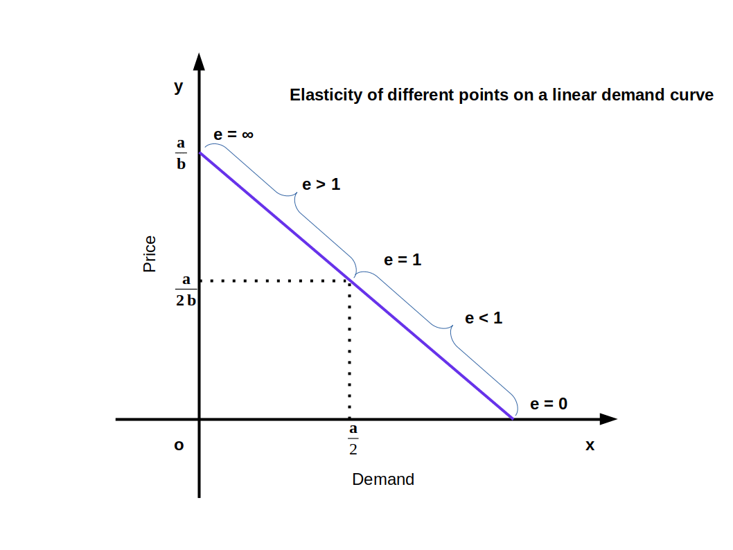
The value of elasticity changes with the change in P and q.
\( {e\,=\,{\frac{-bP}{a\,-\,bP}}} \) (-b = 2, a = 20, P = 5)
\( {e\,=\,{\frac{-2×5}{20\,-\,2×5}}} \)
\( {e\,=\,{\frac{-10}{20\,-\,10}}} \)
\( {e\,=\,{\frac{-10}{10}}} \) = -1 │e│ = 1
Geometric measure of elasticity
We can easily find out the elasticity of different points on a linear demand curve that touches at x- axis and y-axis- by using the geometric method. In this method we divide the lower segment of the linear demand curve with the upper segment.
$$ {\mathbf{e\,=\,{\frac{lower\, segment}{upper\, segment}}}} $$
In the above Diagram, C is a point on the demand curve AB. The length of the lower segment, CB is 4cm and that of the upper segment AC is also 4cm. Therefore,
$$ {{e\,=\,{\frac{lower\, segment}{upper\, segment}}}} $$
$$ {{=\,{\frac{4}{4}}}} = 1 $$
We get price elasticity of demand as 1.

3. Expenditure method
The expenditure is calculated by multiplying price and quantity demanded, i.e., E = pq. Under expenditure method the elasticity is determined by comparing the change in price and the change in expenditure. In this method we can find whether elasticity is more than one, unitary, or less than one.
- If price and expenditure move in the opposite direction, elasticity will be more than one. When price increases expenditure decreases, and when price decreases, expenditure increases.
- When price changes and expenditure remains unchanged, elasticity will be one or unitary. i.e., there is no change in expenditure though price changes.
- If price and expenditure move in the same direction elasticity will be less than one. i.e., when price rises, expenditure also rises, and when the price falls, expenditure also falls. The relation between price; expenditure and elasticity is given in below Table.
| Table 2.1 Expenditure Method | |||
| Price | Quantity | Expenditure | Elasticity |
|---|---|---|---|
| 10 | 5 | 50 | e > 1 |
| 15 | 3 | 45 | |
| 10 | 6 | 60 | e = 1 |
| 15 | 4 | 60 | |
| 10 | 7 | 70 | e < 1 |
| 15 | 6 | 90 | |
Constant Elasticity Demand Curve
Elasticity of a linear demand curve can be any value from 0 to ~. But in some demand curves elasticity will be constant at all points. Whatever may be the changes in price, quantity demanded is unaffected is called constant elasticity of demand.
Above given Diagram shows a vertical demand curve that indicates perfectly inelastic demand. Any point on this curve would always have 0 elasticity.
Similarly, all points on the rectangular hyperbola demand curve will have unitary elastic demand as shown in the above given Diagram.
Factors Determining Price Elasticity of Demand for a Good
Price elasticity of demand is influenced by several factors. They are briefly described below:
- Nature of the good: Elasticity of a good depends on whether it is a necessary or a luxury. If it is a necessary good elasticity would be low. If it is a luxury good it will have a high elastic demand.
- Availability of close substitutes: Substitute goods will always have highly elastic demand, while non- substitute goods will have inelastic demand.
- Proportion of income spent on the good: Consumers usually spend only a small portion of their income on certain goods like salt, match, etc. Elasticity of these goods will be low.
- Income of the consumer: As far as high income consumers are concerned elasticity of demand of most of the goods they use will be low. But the goods used by the poor would have high elasticity.
- Price of the good: Elasticity of demand for cheap goods will be low, and that of expensive and luxury goods would be high.
- Time period: Elasticity is high for long period compared to short period. This is because consumer can control consumption, during long period, by switching over to cheap substitutes.
![]()
0 Comments