Plus One Economics Chapter 13
Chapter 13 :-
Organisation of Data

Introduction The data collected in its original form is unorganised. Hence we call it raw data. This raw data is to be organised or classified so that it will become meaningful for the purpose of further statistical analysis.
Have you ever observed sorting of letters in a post office? Letters collected in a post office are sorted into different lots on a geographical basis. They are then put in separate bags, each containing letters with a common characteristic, viz., having the same destination. In other words, they are classified to form groups of homogeneous character. Similarly, when you arrange your books in a certain order, it will be easier for you to handle them. You may group (classify) them according to subjects. In such a case, each subject becomes a group or a class. If you require a book, say, Economics I, what you should do is to search for that book on the group ‘Economics’. Otherwise, you have to search through the entire books to find the particular book you require. The activity taking place in the above instances is what is called classification Similarly, the raw data collected have to be organised or classified to make them useful for statistical interpretation.Raw Data The data collected in its original form is highly disorganised. They are often very large and cumbersome to handle. It is a tedious task to draw meaningful conclusions from such a raw data, Therefore, proper organisation and presentation of such data is required before any systematic statistical analysis is undertaken. Hence, after collecting data, the next and the most important step is to organise and present them in a classified form.
Suppose you want to know the performance of students in Economics I. You collected data on marks in Economics I of 100 students of your school. The data presented on a table will appear as follows:| Table 13.1 Marks in Economics 1 of 100 Students | |||||||||
|---|---|---|---|---|---|---|---|---|---|
| 46 | 44 | 11 | 10 | 50 | 55 | 48 | 36 | 88 | 41 |
| 61 | 58 | 57 | 56 | 57 | 48 | 54 | 57 | 100 | 40 |
| 43 | 69 | 63 | 60 | 59 | 58 | 59 | 64 | 65 | 51 |
| 65 | 29 | 37 | 51 | 54 | 55 | 71 | 81 | 57 | 91 |
| 70 | 50 | 52 | 49 | 48 | 49 | 70 | 71 | 54 | 54 |
| 48 | 46 | 49 | 54 | 55 | 54 | 60 | 59 | 56 | 66 |
| 49 | 45 | 63 | 63 | 62 | 61 | 59 | 59 | 49 | 65 |
| 65 | 41 | 26 | 25 | 24 | 27 | 18 | 24 | 39 | 23 |
| 45 | 52 | 45 | 44 | 43 | 45 | 46 | 12 | 24 | 34 |
| 47 | 45 | 58 | 57 | 59 | 58 | 59 | 60 | 74 | 24 |


Classification of Data Classification of data stands for grouping of related facts into classes. Facts in one class differ from those of another class with respect to some characteristics they possess. These characteristics form the basis of classification. Groups or classes of a classification can be done in many ways.
Objectives of Classification
To condense the data for easy understanding
To help comparison
To eliminate unnecessary details
To make decision making possible
To enable further statistical treatments
To identify main features of the data
Types of Classification
Data can be classified on the following four basis:
Geographical, i.e., area wise
Chronological, i.e., on the basis of time
Qualitative, i.e., according to some attributes
Quantitative, i.e., in terms of magnitudes

i. Chronological Classification
It is the arrangement of data in ascending or descending order with reference to time. When data are observed over a period of time the type of classification is known as chronological classification. For example, population of India may be observed for a number of years and shown timewise.
| 13.2 Chronological Classification | |
|---|---|
| Year | Population |
| 2009 | 567 |
| 2010 | 638 |
| 2011 | 736 |
| 2012 | 758 |
ii. Geographical Classification
In this type, data are classified on the basis of geographical differences between the various items. It is also called spatial classification. For example, population on India can be shown state wise. This is a geographical classification.
It is the arrangement of data with reference to geographical location such as countries, states (Spatial). Production of rice in different states of India is given in below table.
| 13.3 Geographical Classification | |
|---|---|
| States | Production of Rice |
| Andhrapradesh | 1200 |
| Tamilnadu | 950 |
| Kerala | 830 |
iii. Qualitative Classification
Under this method, data are classified on the basis of some qualities or values or attribute such as sex, colour of hair, literacy, religion, etc. They are not measurable. Their presence or absence can only be known.
Classification according to attributes may be (a) simple or (b) manifold. In simple classification, data are divided on the basis of only one attribute. For example, the population under study may be divided into two categories on the basis of sex as male and female. In manifold classification, data are divided on the basis of more than one attribute. For example, population of India divided on the basis of sex and literacy, so that there are four groups: (1) male literate, (2) male illiterate (3) female literate and (4) female illiterate.| 13.4 Qualitative Classification | |
|---|---|
| States | Literacy |
| Kerala | 99.5% |
| Karnataka | 95.6% |
| Bihar | 68% |
iv. Quantitative Classification
Quantitative classification refers to the classification of data according to some quantitative measurement, such as height, weight, etc.
| 13.5 Quantitative Classification | |
|---|---|
| Companies | Sales |
| Hundai | 800 |
| Tata | 638 |
| Maruti | 736 |
 Quantitative Data:
Data can be measured numerically-eg; Income, Production, Price, Cost..
Qualitative:
Data cannot be measured numerically– eg; Health, Intelligence, Ability..Also termed as Attributes.
Before discussing the process of classification, let us consider certain terms which are commonly used in our study.
Variables and Attributes
Variation is the order of the day. People have different life styles, habits, physical features, age, income, etc. Characteristics like height, weight, etc., are called quantitative characteristics while characteristics like sex, colour of hair, literacy, religion, etc., are called qualitative characteristics. A characteristic that can be measured numerically is called a quantitative characteristic. A characteristic that cannot be numerically measured but can only be expressed on the basis of quality or attributes is called qualitative characteristic. A quantitative characteristic which varies from unit to unit is a variable or variate. Thus weight, height, etc., are variables. Here we shall discuss the variation in characteristics which can be expressed quantitatively.
Continuous and Discrete Variables
In the last chapter you have learnt the term variable. But it does not tell you how it varies. Variable is that characteristic whose value is capable of changing from unit to unit. Suppose, the weight of one of the students in a class is 45 k.g. and of another student. 52 k.g, Now the quantitative characteristic, i.e., weight, changes its value from unit to unit. Hence weight is a variable.
Different variables vary differently. In other words, they differ on the basis of Specific criterion. They are broadly classified into two:- CONTINUOUS
- DISCRETE

Statistical Series : When the items collected are arranged according to some logical order, it becomes a series, Statistical series may be divided into three types on the basis of their construction:
- Individual series.
- Discrete series.
- Continuous series.

Indivisual Series (Simple Array) In this type the items are listed singly, showing the observations relating to them. Each value of the variable occurs usually once. It can be arranged either in ascending or descending order. It may also be called a simple array. For example, the wages earned by 3 workers a day can be shown in an individual series as follows:
| 13.6 Individual Series | |
|---|---|
| Number of workers | Wage (Rs) |
| 1 | 500 |
| 2 | 600 |
| 3 | 550 |
Discrete Series (Frequency Array) Certain items occur many times in the data. Items are arranged indicating the number of times each item occurs (ascending or descending order). A discrete series is also called a frequency array. In discrete series, statistical unit is either not divisible or is not divided. Each class is distinct and different from other class.
| 13.7 Discrete Series | |
|---|---|
| Number of Children per couple | Number of Couples (Frequency) |
| 0 | 21 |
| 1 | 19 |
| 2 | 10 |
| Total | 50 |
Continuous Series In continuous series, different values of the variable are stated in a continuous manner with respect to their frequencies. In continuous series the statistical unit is capable unit, is capable of division and can be measured in fractions of any Size. They are expressed in class interval, and are continuous from beginning to end.
| 13.8 Continuous Series | |
|---|---|
| Marks (Class) | Number of Students (Frequency) |
| 0 – 10 | 5 |
| 10 – 20 | 10 |
| 20 – 30 | 17 |
| 30 – 40 | 13 |
| 40 – 50 | 5 |
| Total | 50 |
The Array
The first step in the organising raw data is to arrange them by their magnitude. A mass of raw data when put into an orderly arrangement by magnitude (ascending or descending order) is called an array. The following example will make you clear this.
Suppose, the raw data obtained from a business unit with regard to the daily wages in rupees of 20 workers are as follows:34, 41, 47, 32, 46, 49, 42, 43, 52, 50
The raw data when arranged in ascending and descending order is shown below:
| 13.9 Array in Ascending Order | |
|---|---|
| Rs | Rs |
| 20 | 36 |
| 21 | 39 |
| 23 | 41 |
| 27 | 42 |
| 30 | 43 |
| 31 | 46 |
| 32 | 47 |
| 33 | 49 |
| 34 | 50 |
| 35 | 52 |
| 13.10 Array in Descending Order | |
|---|---|
| Rs | Rs |
| 52 | 35 |
| 50 | 34 |
| 49 | 33 |
| 47 | 32 |
| 46 | 31 |
| 43 | 30 |
| 42 | 27 |
| 41 | 23 |
| 39 | 21 |
| 36 | 20 |
A look at the arrayed figure in Table 9 or 10 gives us information with respect to the lowest wage (Rs. 20) and the highest wage (Rs. 52). We also know that the range (deviation) between the lowest and the highest wage is Rs. 32 (Rs.52 – Rs. 20). We also notice a concentration of wage between Rs. 30 and Rs. 40.
An array is useful when the number of items in the raw data is small. But if the items are hundreds or thousands, it is very difficult to handle them, and is time consuming, Hence it necessitates the condensation of data. And that is the second step in the organising data. Here condensation or simplification of data is done through a process of classification into groups or classes.The Frequency Array
While making an array it is possible that some values occur frequently. The number of times a value of item occurs in a series is called the frequency. If we mark the number of times a value appears in the series, we will get what is known as frequency array. The frequency array is useful only when the number of items in the raw data is small. The frequency array exhibits the frequency of observations and indicates the concentration of items around certain values.
Let us arrange the following raw data of daily wages (in rupees) of 20 employees in a factory into a frequency array.56, 54, 54, 50, 54, 56, 55, 54, 50, 56
| 13.11 Frequency Array | |
|---|---|
| Daily Wages | No. of Employees |
| 50 | 6 |
| 54 | 6 |
| 55 | 3 |
| 56 | 4 |
| 57 | 1 |
| Total | 20 |
Frequency Distribution
A frequency distribution is an orderly arrangement of data classified according to the magnitude of observations. When data are grouped into classes of appropriate size indicating the number of observations in each class we get a frequency distribution. For example, the students of a college may be classified according to weight as follows:
| 13.12 | |
|---|---|
| Weight (in Kg) | No. of Students |
| 40 – 45 | 40 |
| 45 – 50 | 110 |
| 50 – 55 | 35 |
| 55 – 60 | 240 |
| 60 – 65 | 355 |
| 65 – 70 | 20 |
| Total | 800 |
There are two elements, viz., (1) the variable, i.e., the weight and (2) the frequency.

Construction of Frequency Distribution
Selection of Class
- There is no hard and fast rule to determine number of classes
- A class should not be too big or too small
- There should not be too much classes or too short
- The class limits are the lowest and the highest values that can be included in the class.
- It is the two ends of a class.
- In class 20 – 30, 20 is called the lower class limit and 30 is called upper class limit.
- It is the difference between the upper and lower class limits.
- Class interval is also known as class width or class size.
- The class interval of the class 50 – 100 is 50 (100 – 50 = 50)
- It is the middle value of a class. It is also known as mid value or class mark.
- It lies half way between the lower and upper class limits of a class.
 Magnitude of Class Interval
- The difference between lower and upper class boundaries is called the magnitude of a class interval
- The number of observation corresponding to a particular class is known as the class frequency.
Construction of Frequency Distribution
The following technical terms are important when a frequency distribution is formed:
- Selection of class: The quality of a frequency distribution is determined by a wise choice of the number of classes. There is no hard and fast rule to determine the number of classes. Ordinarily, a frequency distribution should to contain more than 20 to 25 classes and not less than 6 to 8 classes depending on the total number of items of the series. Suppose, in an example, 100 entries are given and the lowest value is 3 and the highest 96. In such a case we can have 10 classes as 0-10, 10-20……..:…..90 – 100.
- Class limits: The class limits are the lowest and the highest values that can be included in the class. For example, if we take the class of 20 – 30, the lowest value 20 is the lower limit and 30, the upper limit.
- Class intervals: The difference between the upper and lower limits is known as class interval. In a class 100-200, the class interval is 100 {i.e., 200 minus 100).
- Class mid-point or class mark: It is the value lying half-way between the lower and upper class limits of a class interval. Class mark = 1/2 (lower limit + upper limit).
- Magnitude of class interval: The difference between lower and upper class boundaries is called the magnitude of a class interval.
- Class frequency: The number of observation corresponding to a particular class is known as the frequency of that class or the class frequency.
How to find Frequency of distribution ?
We had seen that frequency means the number of times a value or item occurs and we have to count the number of times each value of the variable is repeated in the data to get the frequency. If the data is large, the counting simply will invite errors. For this we use the method of tally marks. Tally marks are vertical bars (/) used for counting.
Using tally marks, we can create a frequency distribution. For that first we will draw a table with three columns. In the first column we write the class, in the second we write tally marks, and in the third frequency. All the entries in the first column are filled with classes. Now look at the data given. The first entry is 70. That-will fall in the class 70 – 80. Now strike off the entry 70 in the data and and put a tally mark in the second column right to the class 70 – 80. The second entry is 54. That will fall in the class 50 – 60. Now strike off the entry 54 in the data and put a tally mark in the second column right to the class 50 – 60. This process will be repeated up to when all the entries in the data gone stroked off. One more thing to notice is that, after placing 4 tally marks vertically, for the fifth we put the tally mark horizontally to cut the first four tally marks, so that this gives us a block of 5. For the sixth we put another tally mark vertically leaving some space from the first block. Look at the given below table, it is completed by doing the above said process.
| 13.13 Frequency Distribution with Tally Mark | ||
|---|---|---|
| Class | Tally Marks | Marks |
| 0 – 10 | //// / | 6 |
| 10 – 20 | /// | 3 |
| 20 – 30 | //// //// //// //// //// | 25 |
| 30 – 40 | //// //// //// / | 16 |
| 40 – 50 | //// //// //// //// | 19 |
| 50 – 60 | //// //// /// | 13 |
| 60 – 70 | //// | 5 |
| 70 – 80 | //// /// | 8 |
| 80 – 90 | //// | 4 |
| 90 – 100 | / | 1 |
| Total | 100 | |
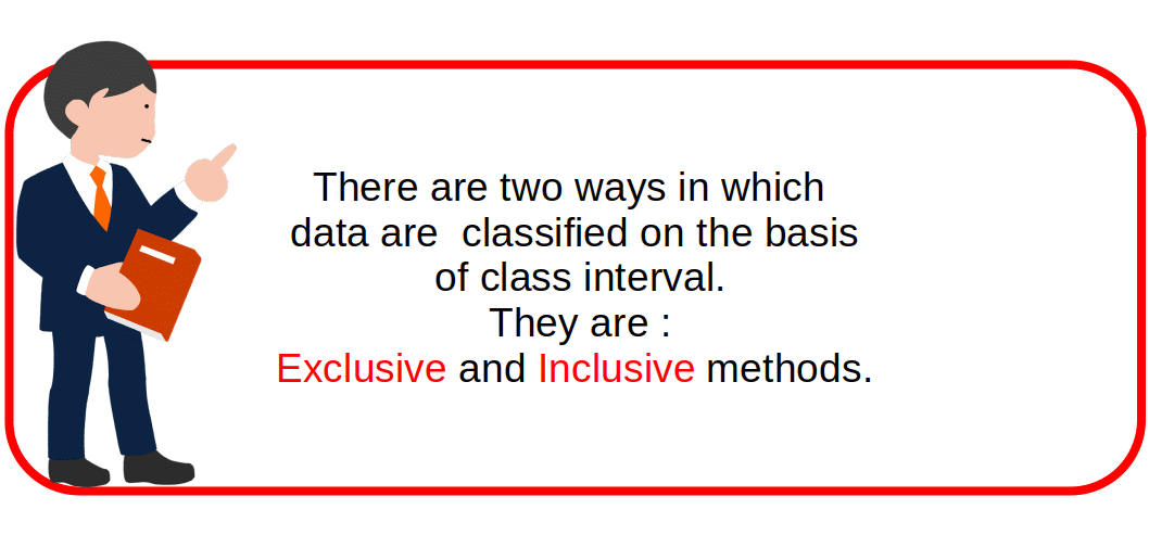
Exclusive Method
When the class intervals are so fixed that the upper limit of one class is the lower limit of the next class, it is known as the exclusive method of classification. The classes are, for example, written as 5-10, 10-15, etc. Here a frequency of 10 is not included in the first class 5-10. It is included in the class 10-15 (Second class).
| 13. 14 Exclusive Classes | |
|---|---|
| Marks (Class) | |
| 0 – 10 | |
| 10 – 20 | |
| 20 – 30 | |
Inclusive Method
Under the inclusive method of classification the upper limit of one class is included in that class itself. The class under this method are written, for example, as 5-9, 10-14, etc. Here a frequency 9 is included in the first class 5-9.
| 13.15 Inclusive Classes | |
|---|---|
| Marks (Class) | |
| 0 – 9 | |
| 10 – 19 | |
| 20 – 29 | |
How to Convert Inclusive Classes into Exclusive Classes ?
Find the difference between the upper limit of a class and the lower limit of the next class. Find half the difference. Subtract this number from all the lower limits and add this number to all the upper limits.
| 13.16 Inclusive Classes | |
|---|---|
| Marks (Class) | |
| 0 – 9 | |
| 10 – 19 | |
| 20 – 29 | |
Difference between the upper limit of a class and the lower limit of the next class = 10 – 9 = 1
Half the difference : \( {{\frac{ 1}{2}} } \) or (0.5).
Now we can get exclusive type class as given below.
| 13.17 Exclusive Classes | |
|---|---|
| Marks (Class) | |
| -0.5 – 9.5 | |
| 9.5 – 19.5 | |
| 19.5 – 29.5 | |
Cumulative Series
In a cumulative series the frequencies are progressively totalled and aggregates are shown.
| 13.18 Cumulative Series | |
|---|---|
| Marks (Class) | Number of Students (Frequency) |
| Marks below 10 | 12 |
| ” below 20 | 18 |
| ” below 30 | 24 |
| ” below 40 | 30 |
| ” below 50 | 36 |
The cumulation may be upward or downward.
Loss of Information When we classify data into a frequency distribution there is an inherent shortcoming. When it summarises the raw data to make it concise, it fails to give all details that are found in raw data. That is, while summarising it as a classified data, there is a loss of information. We noted that once the data are grouped into classes, an individual observation has no significance in further statistical computations. Consider an example of a class 30 – 40 containing 6 observations, 35, 35, 30, 32, 35 and 38. When we use the frequency table for further analysis, we will not attach any importance to the actual value of the items. We consider only the total number of items (6). All values in the class are taken to be equal to the middle value of the class interval (i.e., 35); individual values are not considered. This is true for other classes as well. Thus the use of mid value of each class in place of actual values of the observations in statistical methods involves considerable loss of information.
Open end Class
If the lower limit of the first class or upper limit of the last class are not given, such series are called open end class series.
| 13.19 Open end Class | |
|---|---|
| Marks (Class) | Number of Students (Frequency) |
| Marks below 10 | 4 |
| 10 – 20 | 6 |
| 20 – 30 | 6 |
| 30 – 40 | 9 |
| 40 and above | 5 |
Unequal Class
We are now familiar with frequency distributions of equal class intervals. But in some cases, frequency distributions with unequal class intervals will be more appropriate. If all classes in the distributions are not equal, it can be called unequal class distribution. Observe the frequency distribution given below:
| 13.20 Frequency distribution of Marks in Economics | ||
|---|---|---|
| Marks (Class) | Mid Value | Number of Students (Frequency) |
| 0 – 10 | 5 | 2 |
| 10 – 20 | 15 | 8 |
| 20 – 30 | 25 | 5 |
| 30 – 40 | 35 | 6 |
| 40 – 50 | 45 | 24 |
| 50 – 60 | 55 | 18 |
| 60 – 70 | 65 | 20 |
| 70 – 80 | 75 | 7 |
| 80 – 90 | 85 | 6 |
| 90 – 100 | 95 | 4 |
In the above frequency distribution we notice that most of the observations are concentrated in classes 40 – 50, 50 – 60 and 60 – 70. Frequencies corresponding to these classes are 24, 18, 20 respectively. This means that majority of items (62) are highly concentrated around these three classes. This implies that 62 per cent are in the middle range of 40 – 70. Only 38 per cent of data are in other seven classes. These seven classes are sparsely populated. Further we notice that observations in these classes deviate more from their respective class marks than in comparison to those in other classes. Hence making small classes will be more suitable in this case. Unequal class interval is more appropriate to the above frequency distribution.
What we are going to do is that the class with highest concentration ( 40 – 50, 50 – 60 and 60 – 70) are split into two classes. The class 40 -50 into 40 – 45; 45 – 50, class 50 – 60 into 50 – 55; 55 – 60 and class 60 – 70 into 60 – 65; 65 – 70. We retain the other classes as was done earlier (i-e., class interval with 10).| Total number of students in class | 40 – 50 | = 24 |
|---|---|---|
| “ | 40 – 45 | = 11 (assumed) |
| “ | 45 – 50 | = 13 (assumed) |
| “ | 50 – 60 | = 18 |
| “ | 50 – 55 | = 8 (assumed) |
| “ | 55 – 60 | = 10 (assumed) |
| “ | 60 – 70 | = 20 |
| “ | 60 – 65 | = 9 (assumed) |
| “ | 65 – 70 | = 11 (assumed) |
The new classification along with frequency class marks is given in the following table. The new class mark values are more representative of the data in these classes than the old values.
| 13.21 Frequency distribution of unequal classes | ||
|---|---|---|
| Marks (Class) | Mid Value | Number of Students (Frequency) |
| 0 – 10 | 5 | 2 |
| 10 – 20 | 15 | 8 |
| 20 – 30 | 25 | 5 |
| 30 – 40 | 35 | 6 |
| 40 – 45 | 42.5 | 11 |
| 45 – 50 | 47.5 | 13 |
| 50 – 55 | 52.5 | 8 |
| 55 – 60 | 57.5 | 10 |
| 60 – 65 | 62.5 | 9 |
| 65 – 70 | 67.5 | 11 |
| 70 – 80 | 75 | 7 |
| 80 – 90 | 85 | 6 |
| 90 – 100 | 95 | 4 |
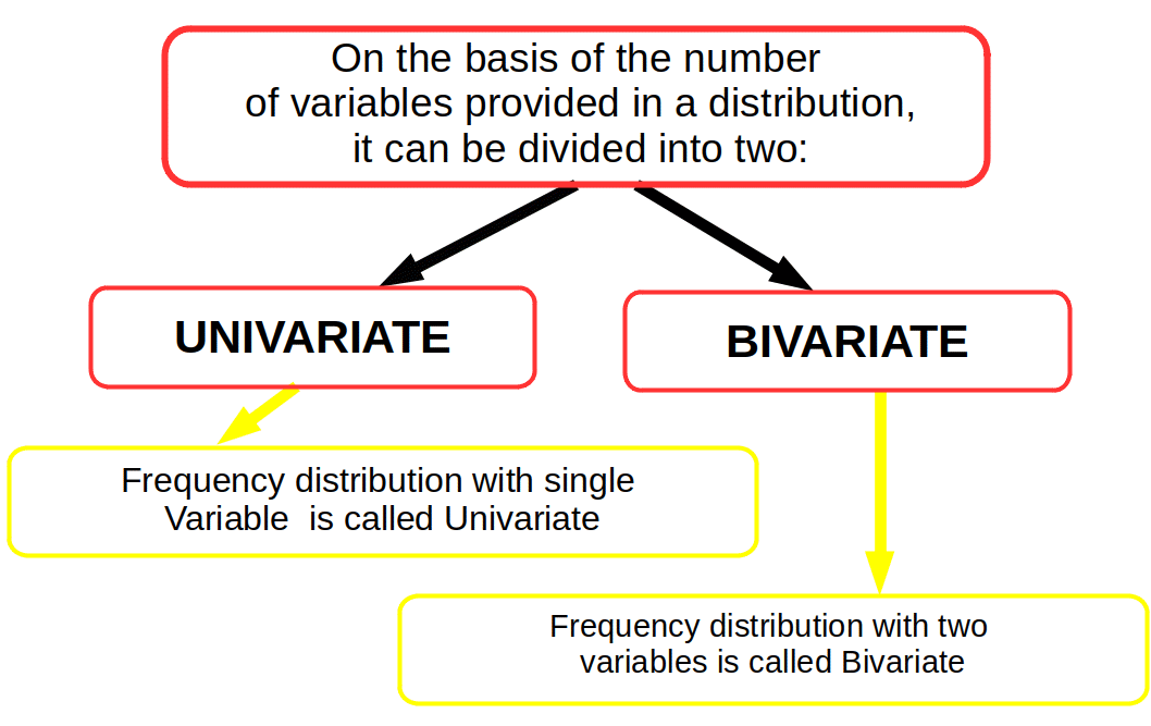
Univariate Distribution.
The frequency distribution of a single variable is called a univariate frequency distribution. The data given in example (inclusive method) shows the univariate distribution of the single variable ‘number of students’.
| 13.22 Univariate Distribution | |
|---|---|
| Marks. | Number of Students. |
| 40 – 50 | 5 |
| 50 – 60 | 8 |
| 60 – 70 | 15 |
| 70 – 80 | 20 |
| 80 – 90 | 7 |
| 90 – 100 | 2 |
Bivariate Distribution.
A bivariate frequency distribution ts the frequency distribution of two variables.
The following table shows the frequency distribution of two variables. Two yariables are sales and advertisement expenditure. The values of variable sales are given in columns and the values of variable advertisement expenditure are shown in rows.| 13.23 Bivariate distribution | ||||
|---|---|---|---|---|
| Sales. | 100 – 200 | 200 – 300 | 300 – 400 | 400 – 500 |
| Cost. | ||||
| 40 – 50 | 5 | 3 | 2 | 1 |
| 50 – 60 | 8 | 4 | 3 | 1 |
| 60 – 70 | 8 | 3 | 1 | 1 |
| 70 – 80 | 6 | 1 | 2 | 1 |
| 80 – 90 | 4 | 1 | 1 | 2 |
![]()
0 Comments