Plus One Economics-Chapter 14

Introduction

After collecting the data by using various methods, the next step is to present them in a systematic manner. This is because raw data itself will not convey their full meaning (The collected data in any statistical investigation are known as raw data). Data when arranged in a systematic manner will bring out their underlying characteristics so that they can be easily understood by the readers.

There are three methods of presenting data:

• (1) Textual or descriptive presentation
• (2) Tabular presentation
• (3) Graphic and diagrammatic representation

In textual presentation, data are presented in a text form. This type of presentation is ideal when data are not voluminous. Look at the following cases:

Case 1

In Hartal day on July 7^th 2008 protesting the hike in bus fare, 15 buses were plying while 240 buses were not operating; 6 shops were opened and all other 345 shops were closed; 3 educational institutions were closed and remaining 39 were found open in Thrissur town.

Case 2

Census of India 2001 reported that Indian population has risen to nearly 102 crores of which 49 crore were females while 53 crore males. 74 crore people resided in rural areas and only 28 crore lived in cities and towns. Non-worker population accounts for 62 crore against 40 crore worker population. Workers out of a 74 crore rural population.

Below given pictures are examples for textual presentation.

This is the systematic arrangement of data in rows and columns. This method of presentation helps to simplify and facilitate comparison of data.

Table 4.1 Rural – Urban composition [ 1971-2001 ]
Year	Rural	Urban
1971	80	20
1981	78	22
1991	74	26
2001	72	28

The table contains 12 entries in 4 rows in and 3 columns. It is called 4 x 3 table giving information on 12 items in 12 boxes. These boxes are called cells of the table. Each cell gives information about an attribute.

Under this method data are classified on the basis of some attribute or quality such as sex, literacy, religion, nationality, occupation etc. They are not measurable.

Table 4.2 Qualitative Classification
Sex	Location		Total
	Rural	Urban
Male	57.07	80.80	60.32
Female	30.03	63.30	33.57
Total	44.42	72.71	47.53

Under this method data are classified on the basis of characteristics which are quantitative in nature such as age, height, weight, income, production etc. They are measurable.

Table 4.3 Quantitative Classification
Year	Rural	Urban
1971	80	20
1981	78	22
1991	74	26
2001	72	28

Under this method data are classified on the basis of Time. Time may be in hours, days, weeks, months, years etc.

Table 4.4 Temporal Classification
Year	Sale (In lakh)
2007	81.7
2008	86.9
2009	101.4
2010	94.7

When classification is done on the basis of place, it is called spatial classification. The place may be village, town, district, state, country, continent etc.

Table 4.5 Spatial Classification
Country	Export Share
USA	21.8
GERMANY	5.6
UK	5.7
RUSSIA	2.1

• Table number is essential for identifying the table.

• Title gives a description of the contents of the table.

• Units is a brief statement about units of measurement used.

• Stubs are the designations of the rows. It is also called row heading.

• Caption are the designations of the columns. It is also called column heading.

• Body contains the actual data. It is the most important part of a table.

• Foot note is a statement meant for giving clarification.

• Source note indicate the source from where the information is taken.

• Table should be simple and attractive.
• It should suit with the size of the paper.
• The captions and stubs should be arranged systematically.
• Units of measurement should be specified.
• Figures may be rounded off as far as possible.
• It should not be crowded with too much data.

There is no hard and fast rule regarding the construction of a good statistical table. However, the following general instructions may be followed for systematic presentation of data.

1. The table should suit the size of the paper usually with more rows and columns.
2. The captions and stubs should be arranged systematically. This would help in giving stress for more important items and in reading the table with ease. Arrangement of data may be according to size or importance, chronologically, geographically or alphabetically.
3. A rough draft should be prepared before preparing the table. This will help in planning the size and shape of a table.
4. The unit of measurement should be specified, e.g., income in rupees or weights in kilograms, etc.
5. Figures should be rounded off to avoid unnecessary details.
6. To emphasise certain figures, they should be in distinctive type or in a box or circle, or shown in the lines.
7. The table should not be overloaded with so many details.
8. A miscellaneous column should be added to include important items.
9. Abbreviation should be avoided.
10. Indicate a zero quantity by a zero. Zero should not be used to indicate that information is not available. If it is not available, show this fact by letters NA (Not Applicable) or by dash (-).
11. Avoid using ditto marks (,,) in the table.
12. A table should not contain any irrelevant data. It should have only those data which can be placed in relation with other.

Although these guidelines are helpful, as Prof. Bowly rightly points out, “In collection and tabulation, common sense is the chief requisite and experience the chief teacher.”

• Tables contain only numerical data, They do not contain details.
• They can be used only by experts. Common men may not understand them properly.
• Some tables are very large. They cannot facilitate comparison.

This is the more attractive and eye-catching method of presenting data. This provides the quickest understanding of the actual situation to be explained by data in comparison to tabular or textual presentations. The types of diagrams are broadly divided into three:

1. Geometric Diagram.
2. Frequency Diagram.
3. Arithmetic Line Graph.

Bar diagrams are the most common type of diagrams used to indicate changes in magnitude over time or space. A bar is a thick or wide line. It is only the length of the bar which is taken into consideration. Breadth of the bar has no significance, but shown only for attention. Therefore, bar diagrams are also called one-dimensional diagrams. A bar diagram may be set.up in horizontal or vertical form. Bars of a bar diagram can be visually compared by their relative height and accordingly data are comprehend quickly. Data for this can be of frequency type or non-frequency type.

The following points must be kept in mind while constructing bar diagrams.

• The width of the bar should be uniform.
• The space between the bars should be uniform.
• The length of the bars should be proportional to the magnitude of the variables that they represent.
• All the bars should rest on the same line, called the base.

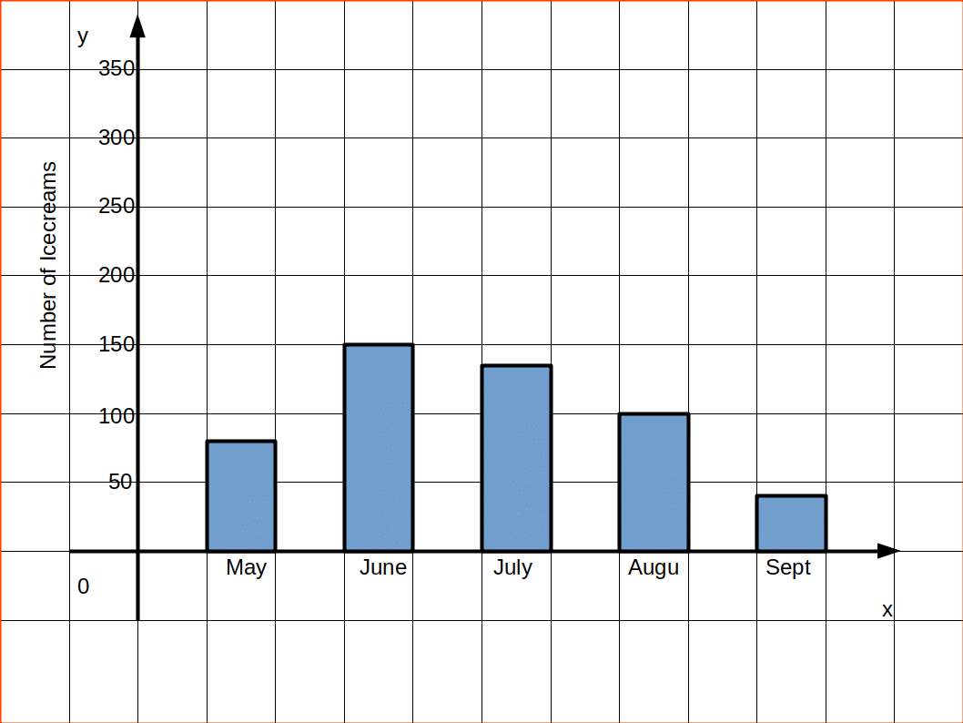
SIMPLE BAR DIAGRAM

Simple bar diagram is used to represent only one variable. It is easy to draw and simple to understand.

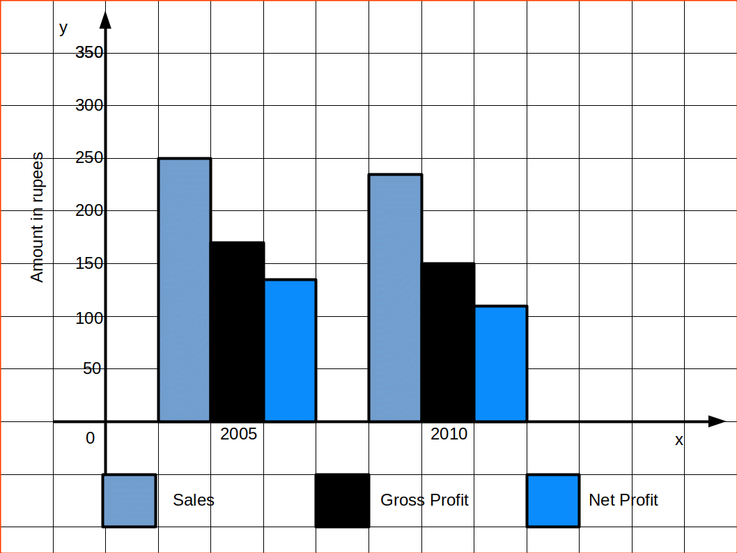
MULTIPLE BAR DIAGRAM

Multiple bar diagram is used for comparing two or more variables. The bars are dawn side by side. In order to distinguish the bars for different variables, it is nice to give different colours or shades to different variables.

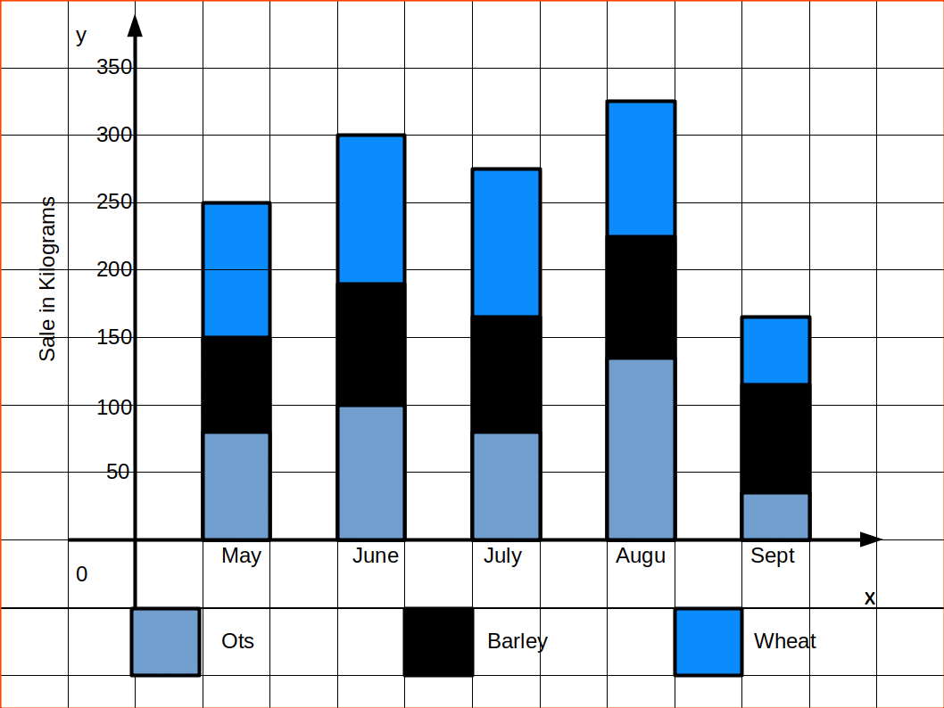
COMPONENT BAR DIAGRAM

In Component bar diagrams, each bar representing the magnitude of a given phenomenon is again sub-divided into various components. Hence it is also called sub-divided bar diagrams. A component bar diagram shows the bar and its sub-divisions into two or more components. Each component occupies a part of the bar proportional to its share in the total. They are very useful in comparing the sizes of different components and also getting an idea about the amount of their contribution.

To construct a component bar diagram, after drawing the base line, a bar is constructed on the line (may be taken as the x-axis) with its height equivalent to the total value of the bar. Then the proportional heights of the components are marked. The rest of the bars are also constructed likewise. Distinguish components by different colours or shades.

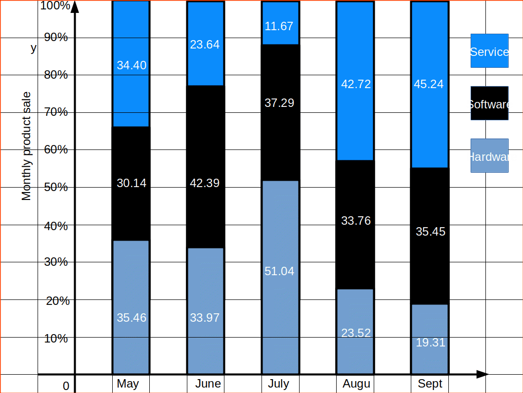
PERCENTAGE BAR DIAGRAM

Percentage bar diagrams are component bar diagrams drawn on the basis of percentage. Hence the total length of each bar will be 100. This will be useful in comparison of relative characteristics. In this case the bars are all of equal height. Each sub-division shows the percentage to the total.

Pie diagram is also a diagrammatic representation of statistical data. Instead of bars, different segments of a circle represent contribution of various components to the total. In a pie-diagram, a circle is divided into component sectors with areas proportional to the size of the corresponding component. This kind of representation is very much useful because it clearly brings out the relative importance of the various components. For constructing a pie diagram, first we draw a circle of any radius. We convert the component values to percentages and then multiply each percentage value by 3.6°. Then divide the circle into various segments according to these angles. This is because, a circle is having in total 360°, and likewise, it is having 100 equal parts of 3.6°. The following illustrations will make the conversions to percentages and then into angles clear. Let us now consider a data from your class room. Suppose that there are 45 students in your class and you had conducted a survey among them to find their mode of transportation to the school. The data obtained may be presented in a pie-diagram.

Let us construct a pie diagram for the following distribution.

Table 4.6 School Transportation
Mode of transport	No. of students
School bus	18
Private vehicle	6
Public transport	12
By walking	9

For constructing the pie diagram, first we have to convert the values to percentages, and then to angles. New table is created as given below.

Table 4.7 School Transportation
Mode of transport	No. of students	Percentage	Angle
School bus	18	\( \mathbf{{{\frac{18 × 100}{45}} }} = 40 \)	40×3.6 = 144º
Private vehicle	6	\( \mathbf{{{\frac{6 × 100}{45}} }} = 13.33 \)	13.33×3.6 = 48º
Public transport	12	\( \mathbf{{{\frac{12 × 100}{45}} }} = 26.67 \)	26.67×3.6 = 96º
By walking	9	\( \mathbf{{{\frac{9 × 100}{45}} }} = 20 \)	20×3.6 = 72º
Total	45	100	360º

Now we can draw a circle with any radius. Measure angles 144º, 48º, 96º, and 72º successively. We can beautify diagram using different colours.

Frequency Diagrams

Data in the form of grouped frequency distributions are generally represented by frequency diagrams. The commonly used frequency diagrams are:

1. Histogram.
2. Frequency Polygon.
3. Frequency Curve.
4. Ogive.

Histogram

Histogram is a two dimensional diagram of a continuous frequency distribution. In a histogram, rectangles are drawn with class intervals as bases and corresponding frequencies as heights. There are no gaps between the rectangles of a histogram. The scale on the x-axis must be continuous. For that, we convert the frequency table into exclusive, if it was not. If only the midpoints of classes are given, then we determine the upper and lower limits properly. This method is used when we are asked to construct histogram for discrete frequency distribution.

While constructing the histogram the class limits are taken on the x-axis and the frequencies on the y-axis. If the frequency distribution is having all its classes with equal class intervals, then the rectangles are drawn with uniform width. Then we get rectangles touching each other and each having class interval as their width and frequency as their height. If the class intervals are not uniform, then the widths of the rectangles also vary. This is because, we have to make an adjustment for the unequal classes. For the adjustment, we take that class with lowest class interval. Let it be c. Take any class whose class interval is not c. Divide the class interval by c. Let the answer be k. Then divide the frequency of the class by k. This will give the new frequency of the class. That is,

k = \( \mathbf{{{\frac{class\,interval\,of\,the\,class}{c}} }} \)

where c = lowest class interval

new frequency = \( \mathbf{{{\frac{frequency\,of\,the\,class}{k}} }} \)

Histogram is used for locating mode of a frequency distribution graphically.

Table 4.8 Histogram and Bar Diagram
Bar Diagram	Histogram
Diagramatic presentation of data	Diagramatic presentation of data
Use of rectangles	Use of rectangles
Considers height only	Considers both height and width
Both for discrete and continuous variables	Only for continuous variables
Some space is left between consecutive bars	No space is left in between two rectangles
Can not locate mode	Can locate mode

Let us draw a histogram for the followuing distribution.

Table 4.9
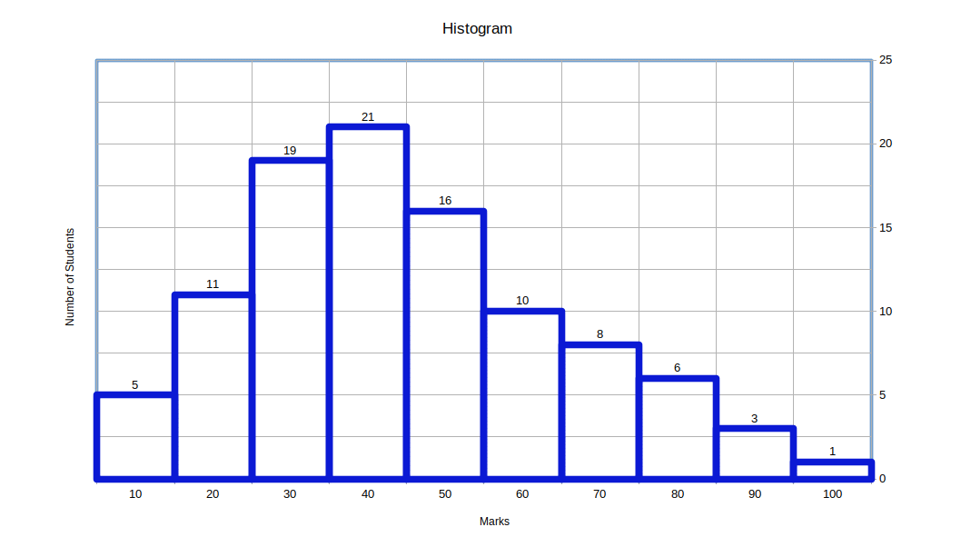
Marks.	Number of Students.
0 – 10	5
10 – 20	11
20 – 30	19
30 – 40	21
40 – 50	16
50 – 60	10
60 – 70	8
70 – 80	6
80 – 90	3
90 – 100	1

We will get a beautiful Histogram like this.

CLASS INTERVALS ARE UNEQUAL

When class intervals are unequal a correction for unequal class-intervals should be made. For making the adjustment, we take that class which has lowest class-interval and adjust the frequencies of other classes. The adjusted frequencies are obtained on dividing the frequency of the given class by the corresponding adjustment factor which is given by

$$ \mathbf{{{\frac{Magnitude\,of\,the\,class}{Lowest \,class \,interval}} }} $$

Let us create a histogram for the following distribution

Table 4.10
Weekly wages ( in ₹ )	Number of Workers.
10 – 15	7
15 – 20	19
20 – 25	27
25 – 30	15
30 – 40	12
40 – 60	12
60 – 80	8

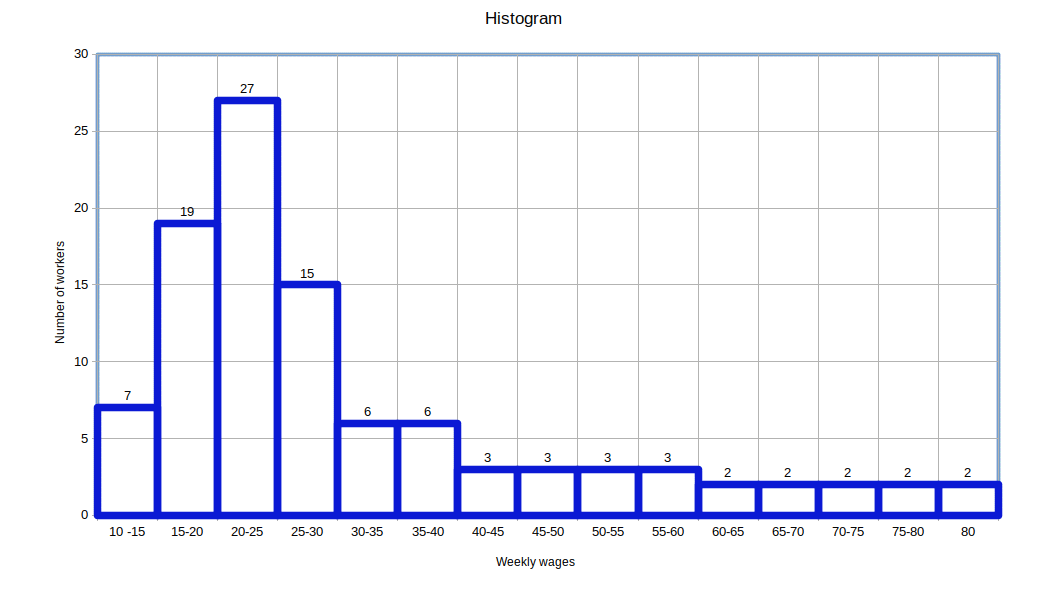
Since class-intervals are not uniform, frequencies should be adjusted. The adjustment is as follows:

The lowest class interval is 5. The frequency of the class 30-40 shall be divided by 2 \( \mathbf{{({\frac{12}{2}} }} = 6) \) since the class interval is double and that of 40-60 by 4 \( \mathbf{{({\frac{12}{4}} }} = 3) \), etc :

Now we can create a table with equal class intervals and adjusted frequencies.

Table 4.11
Weekly wages ( in ₹ )	Number of Workers.
10 – 15	7
15 – 20	19
20 – 25	27
25 – 30	15
30 – 35	6
35 – 40	6
40 – 45	3
45 – 50	3
50 – 55	3
55 – 60	3
60 – 65	2
65 – 70	2
70 – 75	2
75 – 80	2

We will get histogram as given below.

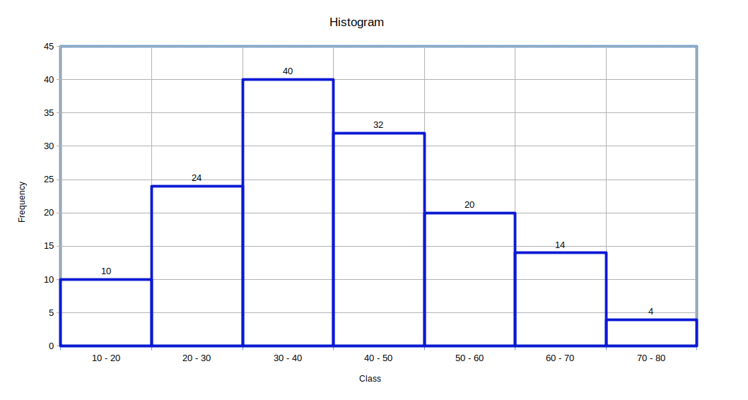
ONLY MID-VALUES ARE GIVEN

When only mid-values are given, ascertain the upper and lower limits of the various clsses and then construct the histogram in the same manner.

Let us create a histogram for the following distribution.

Table 4.12
Mid-value	Frequency.
10	10
25	24
35	40
45	32
55	20
65	14
75	4

Here only the mid-values are given. Now we need to find the lower and upper limits of each class. These classes would be like the below given table.

Table 4.13
Class	Frequency.
10 – 20	10
20 – 30	24
30 – 40	40
40 – 50	32
50 – 60	20
60 – 70	14
70 – 80	4

Now we can create histogram using the rearranged distribution.

Locating Mode Graphically

STEPS

1. Draw a histogram of the given data.
2. Draw two lines diagonally in the inside of the modal class bar, starting from each corner of the bar to the upper corner of the adjacent bar.
3. Then, draw a perpendicular line from the point of intersection to the X – axis, which gives us the modal value.

Let us draw a histogram and find mode for the following data

Table 4.14
Profit	Number of firms
0 – 100	12
100 – 200	18
200 – 300	27
300 – 400	20
400 – 500	17
500 – 600	6

Now we can create a diagram showing how mode is located using histogram.

A histogram may look similar to a bar diagram. But, these two are entirely different, except for the fact that both are diagrammatic representation of statistical data. Their dissimilarity lies in the following facts.

1. In bar diagram there is gap between bars. In histogram there is no gap between rectangles.
2. In bar diagram it is the height and not the width or the area of the bar that is insignificant. In histogram both the height and the width are significant.
3. Bar diagram may be drawn for both discrete and continuous data. But histogram can be drawn only for continuous data.
4. Bar diagram is not used for locating mode of a distribution. But, histogram is used for locating mode of a distribution graphically.

A frequency distribution is a graphical representation of a frequency distribution. It is the most common method of presenting grouped frequency distribution. A polygon is a two dimensional geometric figure formed of three or more straight sides. For constructing a frequency polygon, the class midpoints are marked on the x-axis and frequency on the y-axis. Then frequencies corresponding to each midpoint are plotted and these points are joined by straight lines. The first and the last points plotted are joined to the base line to form a polygon. The rules we had followed for inclusive type frequency distributions and for unequal class intervals while drawing a histogram are very well applicable for frequency polygons also.

A frequency polygon may be drawn from a histogram also. For that, first we draw the histogram of the given frequency distribution as discussed in the above section. Then midpoints of the upper horizontal sides of the rectangles are marked. The adjacent points are joined by straight lines. Midpoint of the upper vertical side of the first rectangle and that of the last rectangle are joined to the base line to form a polygon.

A frequency polygon can be fitted to a histogram for studying the shape of the curve. When comparing two or more distributions plotted on the same axes, frequency polygon is likely to be more useful since the vertical and horizontal lines of the distributions may coincide in a histogram.

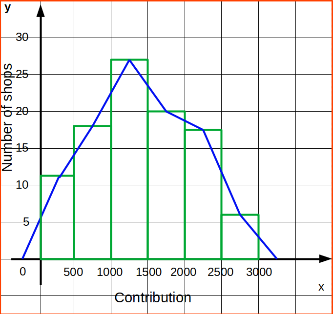
Construction of frequency polygon by drawing histogram

The contribution given in rupees of 100 shops are distributed as follows:

Table 4.15
Contribution	Number of shops.
0 – 500	12
500 – 1000	18
1000 – 1500	27
1500 – 2000	20
2000 – 2500	17
2500 – 3000	6

Let us draw a histogram for the data and show the frequency polygon for it.

Construction of frequency polygon without drawing histogram

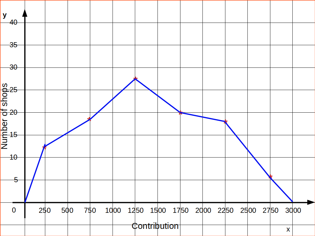
Let us draw a frequency polygon for the following data which give the contribution given by shops.

Table 4.16
Contribution	Number of shops.
0 – 500	12
500 – 1000	18
1000 – 1500	27
1500 – 2000	20
2000 – 2500	17
2500 – 3000	6

Here the distribution is exclusive and class intervals are uniform. For drawing a frequency polygon, first we construct a table with class mid points and corresponding frequencies.

Table 4.17
Mid-value	Frequency.
250	12
750	18
1250	27
1750	20
2250	17
2750	6

Now we draw the x and y axes; and mark the class midpoints on the x-axis and fréquency on the y-axis. For each class midpoint, we plot the corresponding frequencies and finally join the points by straight line segments. The Starting point and the endpoints are then joined to the base line. The frequency polygon for the data is given below:

Histogram may also be used to represent discrete frequency distribution by taking the given values of the variable as the mid points of continuous classes.

We can draw two or three frequency polygons in the same graph paper, but not histogram.

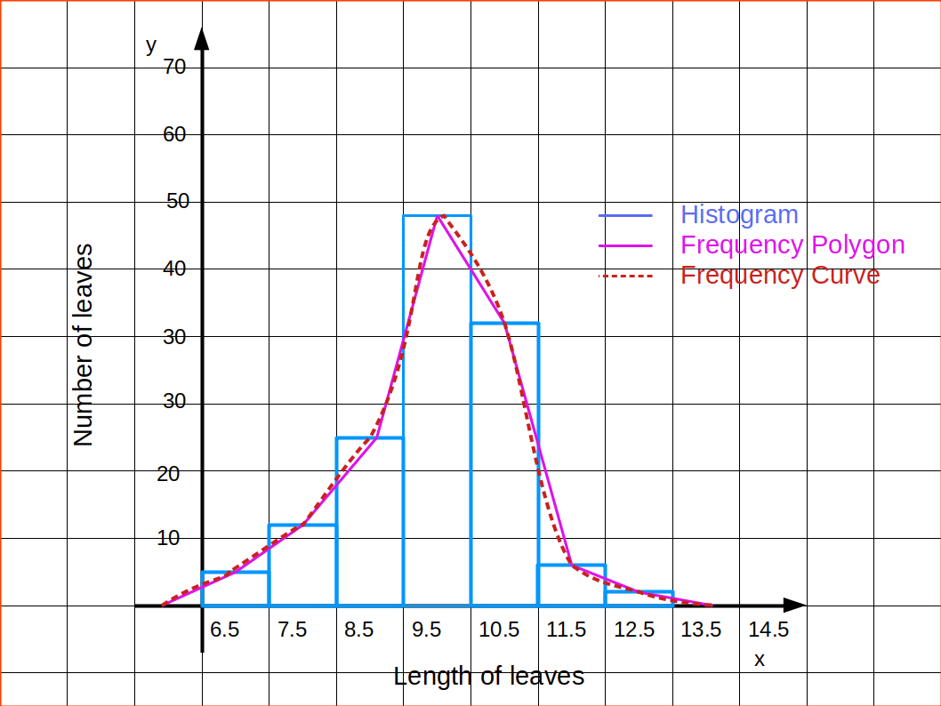
A continuous frequency distribution represented by a smooth curve is known as frequency ‘curve. As in the case of drawing frequency polygon, here also, the class midpoints are taken along the x-axis and frequency along the y-axis. The points thus plotted are joined by a smooth curve. It may not necessarily pass through all the points of the frequency polygon, but it passes through them as closely as possible. The curve is drawn in such a way that the area included under the curve is approximately as that of the frequency polygon.

Frequency curves are used for interpolation. Interpolation is the process of estimating the value of a function that lies between known values, often by means of a graph.

Let us draw a histogram, frequency polygon and frequency curve representing the following data.

Table 4.18
Length of leaves	Number of leaves
6.5 – 7.5	5
7.5 – 8.5	12
8.5 – 9.5	25
9.5 – 10.5	48
10.5 – 11.5	32
11.5 – 12.5	6
12.5 – 13.5	1

Above distribution is shown as frequency curve in the below diagram.

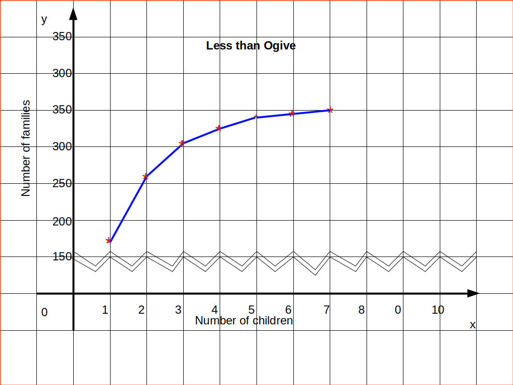
Ogives are frequency curves drawn for cumulative frequencies. Therefore ogives are otherwise called cumulative frequency curves.

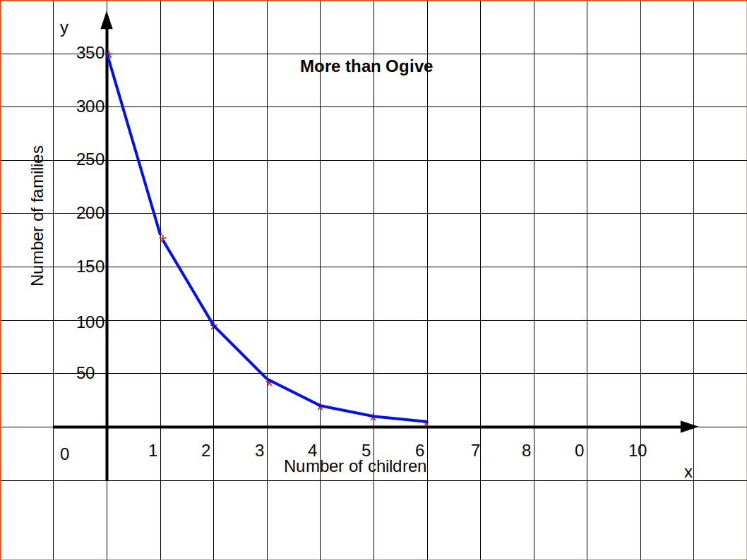
We had studied two types of cumulative frequencies; ‘Less than Cumulative Frequency’ and ‘More than Cumulative Frequency’. The frequency curve drawn using less than cumulative frequencies is known as ‘Less than Cumulative Frequency Curve’ or ‘less than Ogive’, and the frequency curve drawn using more than cumulative frequencies is known as ‘More than Cumulative Frequency Curve’ or ‘more than ogive’. For drawing less than ogives, upper class limits are marked on the x-axis and corresponding less than cumulative frequencies on the y-axis; while for drawing more than ogives, lower class limits are marked on the X-axis and corresponding more than cumulative frequencies on the y-axis. Less than ogive is an increasing graph or rising curve and more than ogive is a decreasing graph or declining curve.

An interesting feature of the ogives is that when we draw them together, their point of intersection will give us the median of the distribution. Median is a measure of central tendency like mode. Ogives can also be used to locate quartile values, deciles or percentiles of a distribution.

Let us draw less than and more than ogives using the following data.

Table 4.19
Number of children	Number of families
0	171
1	82
2	50
3	25
4	13
5	7
6	2

We can arrange the above data in the form of frequency distribution.

Table 4.20
Number of children	Number of families
0-1	171
1-2	82
2-3	50
3-4	25
4-5	13
5-6	7
6-7	2

Now we can arrange data in to less than series.

Table 4.21
Number of children	Number of families
Less than 1	171
” ” 2	253
” ” 3	303
” ” 4	328
” ” 5	341
” ” 6	348
” ” 7	350

Then draw Ogive by less than method.

We can also arrange data in to more than series.

Table 4.22
Number of children	Number of families
0 or more	350
1 ” “	179
2 ” “	97
3 ” “	47
4 ” “	22
5 ” “	9
6 ” “	2

Then draw Ogive by more than method.

We have to draw less than and more than ogive to locate median.

For constructing less than ogive and more than ogive, we want both lower class limits and upper class limits and also both less than cumulative frequencies and more than cumulative frequencies.

Table 4.23
Mid-value	Less than cumulative frequency	More than cumulative frequency
0	—	83
5	2	81
10	7	76
15	13	70
20	21	62
25	34	49
30	51	32
35	62	21
40	70	13
45	75	8
50	79	4
55	82	1
60	83	—

The less than and more than ogives drawn together for the data is given in the below figure.

Arithmetic line graph is a diagrammatic representation of statistical data over a period of time. Hence it is also called time series. In arithmetic line graphs, values of a variable at different periods of time are shown. The graph shows the changes in the values of a variable with the passage of time. Here, time is the independent variable. The variable which varies according to time, such as, total output of agriculture, the consumption, the national income is known as dependent variable. In time series, time is taken along the x-axis and the dependent variable along, the y-axis. Arithmetic line graphs are used to understand the trend, periodicity, etc., in a long term time series data.

Consider the data given below of production of steel in a country from 2000 to 2009

Table 4.24
Year	Production
2000	9.54
2001	10.83
2002	9.12
2003	8.85
2004	10.62
2005	10.85
2006	10.95
2007	11.35
2008	11.65
2009	11.98

Here the dependent variable is the production of steel. So it may be marked along the y-axis and time period along the x-axis. Arithmetic line graph for the above data is given in below diagram.

If the fluctuations in the values of a variable are vary small as compared to the size of the item, a false baseline is used. By using this even minor fluctuations are magnified so that they are clearly visible on the graph. If the size of items is comparatively big and if the vertical scale begins from zero, the curve would be mostly on the top of the paper and if the differences in the values of various items are not much, it would more or less, be of the shape of a straight line. In false base line the scale from zero to the smallest value of the variable is omitted. Whenever false baseline is Used it should be very clearly indicated on the graph. Generally in such cases, vertical scale is broken in two parts and some blank space is left between them. To make the breaking of vertical scale prominent usually saw-tooth lines are used.

• Diagrams are easy to understand.
• Diagrams are more attractive.
• Diagrams are more appealing.
• Diagrams save time and labour of the user.
• It facilitates comparison more quickly