Plus One Economics Chapter 15
Chapter 15 :-
INTRODUCTION:
We had learnt how to present a statistical data precisely and meaningfully. This is to enable the statistician to study the data well and draw inferences from the,‘data. But by presentation only, it cannot be possible. Hence after presenting the data, it should be condensed. Condensation of data is essential in statistical analysis because, a large number of figures not only confusing but difficult to analyse also. In order to reduce the complexity of data and to make them comparable, it is essential that various characteristics which are being compared are reduced to one figure each. If, for example, a comparison is made between the marks obtained by 45 students belonging to Batch-A of plus-1 and 48 students belonging to Batch-B of plus-1 of your school in the first term examination, it would be impossible to arrive at any conclusion, if the two series relating to these marks are directly compared. On the other hand, if each of these series is represented by one figure, comparison would be easier. It is, obvious that a figure which is used to represent a whole series should neither have the lowest value in the series nor the highest value, but a value somewhere between these two limits, possibly in the centre, where most of the items of the series gather. Such a figure is called the average or a measure of central tendency.
The average represents the whole series and as such, its value always lies between the highest and the lowest values and generally it is located in the centre or middle of the distribution. Thus, central tendency summarises the data in a single value in such a way that this single value can represent the entire data. A measure of central tendency is a single figure that is computed from a given series to give a central value about the entire series. Hence a measure of central tendency may be defined as a typical value around which the values of a distribution congregate.
- It should be easy to understand
- It should be simple to compute
- It should be based on all the items
- It should not be unduly affected by extreme items
- It should be rigidly defined
- It should be capable of further algebraic treatment
- It should have sampling stability

- ARITHMETIC MEAN
- Simple Mean
- Combined Mean
- Weighted Mean
- MEDIAN
- MODE

Arithmetic Mean
On the basis of the type of data series that has provided to us (ie, Individual, Discrete, Continuous), it will be convenient if we use appropriate formula for finding averages in each of these series.
There are three methods by which Simple mean can be calculated in each of these three series.
They are :
- Direct Method
- Assumed Mean Method
- Step Deviation Method

Calculation of Arithmetic Mean
Calculation of arithmatic mean can be studied under two heads.
- Arithmetic Mean for Ungrouped Data
- Arithmetic Mean for Grouped Data
Arithmetic Mean for Ungrouped Data
Arithmetic Mean for Ungrouped data can be calculated using the following methods:
- Direct Method
- Assumed Mean Method
- Step Deviation Method
Individual Series

Direct Method
STEPS
- Find the sum of observations (∑X)
- Take the number of observations (N)
- Use the formula \( X̅ = {{{\frac{ΣX}{N}} }} \)
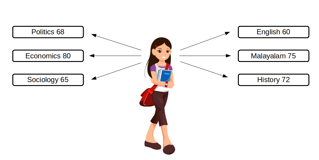 $$ A.M = {{{\frac{60+75+72+68+80+65}{6}} }} $$ $$ = {{{\frac{420}{6}} }} = 70 $$
Assumed Mean Method
STEPS
- Take an assumed mean A
- Take the deviation of each X from the assumed mean. ie., d = X – A
- Find the sum of the deviations to get Σd
- Use the formula \( X̅ = A + {{{\frac{Σd}{N}} }} \) ; where N is the total number of observations
 Let us find the arithmetic mean of the following 20 observations using assumed mean method.
2500, 6500, 3000, 5500, 4500, 6000, 3500, 3000, 5500, 5000, 2000, 4500, 3500, 3000, 4500, 6500, 4000, 3000, 2500, 4500
| Table 5.1 | |
|---|---|
| X | d=X-A=X-4000 |
| 2500 | -1500 |
| 6500 | 2500 |
| 3000 | -1000 |
| 5500 | 1500 |
| 4500 | 500 |
| 6000 | 2000 |
| 3500 | -500 |
| 3000 | -1000 |
| 5500 | 1500 |
| 5000 | 1000 |
| 2000 | -2000 |
| 4500 | 500 |
| 3500 | -500 |
| 3000 | -1000 |
| 4500 | 500 |
| 6500 | 2500 |
| 4000 | 0 |
| 3000 | -1000 |
| 2500 | -1500 |
| 4500 | 500 |
| N=20 | Σd = (-10000)+13000=3000 |
$$=4000 + 150 = 4150 $$
Step Deviation Method
Complexity of calculations in finding arithmatic mean can nfurther be reduced by using step deviation method.
STEPS
- Take an assumed mean A
- Take the deviation of each X from the assumed mean. ie., d = X – A
- Devide the deviation d by common factor c, i.e., \( d ‘ = {{{\frac{d}{c}} }} = {{{\frac{X – A}{c}} }} \)
- Then find Σd’
- Use the formula \( X̅ = A + {{{\frac{Σd’}{N}} }} × c \) ; where N is the total number of observations

45, 30, 65, 70, 40, 25, 45, 25, 55, 40, 20, 50
Assumed mean is taken as 50.
Let c = 5 (we decide value of c only after seeing the column for d in the table)
| Table 5.2 | ||
|---|---|---|
| X | d=X-A=X-50 | \( \mathbf {d ‘ = {{{\frac{d}{c}} }} = {{{\frac{d}{5}} }}} \) |
| 45 | -5 | -1 |
| 30 | -20 | -4 |
| 65 | 15 | 3 |
| 70 | 20 | 4 |
| 40 | -10 | -2 |
| 25 | -25 | -5 |
| 45 | -5 | -1 |
| 25 | -25 | -5 |
| 55 | 5 | 1 |
| 40 | -10 | -2 |
| 20 | -30 | -6 |
| 50 | 0 | 0 |
| N = 12 | Σd’ = (-26) + 8 =-18 | |
$$ X̅ = A + {{{\frac{Σd’}{N}} }} × c = {50+\frac{-18}{12}} × 5 $$
$$= 42.5 $$
Arithmetic Mean for Grouped Data
Discrete Series
Direct Method
STEPS
- Multiply the frequency against each observation with the value of observation to get fx
- Add the column of fx to get Σfx
- Use the formula \( X̅ = {{{\frac{Σfx}{Σf}} }} \)

| Table 5.3 | |
|---|---|
| Income | Number of Persons |
| 1200 | 2 |
| 1500 | 10 |
| 1800 | 15 |
| 2000 | 7 |
| 2300 | 5 |
| 2600 | 4 |
| 3400 | 3 |
| 4200 | 3 |
| 5000 | 1 |
Now we can create a table to find fx.
| Table 5.4 | ||
|---|---|---|
| Income | Number of Persons | fX |
| 1200 | 2 | 2400 |
| 1500 | 10 | 15000 |
| 1800 | 15 | 27000 |
| 2000 | 7 | 14000 |
| 2300 | 5 | 11500 |
| 2600 | 4 | 10400 |
| 3400 | 3 | 10200 |
| 4200 | 3 | 12600 |
| 5000 | 1 | 5000 |
| Σf = 50 | Σfx = 108100 | |
$$ X̅ = {{{\frac{Σfx}{Σf}} }} = {\frac{-108100}{50}} $$
$$= 2162 $$
Assumed Mean Method
Assumed mean method is applying just to simplify the calculations.
STEPS
- Take an assumed mean A
- Take the deviation ‘d’ of each X from the assumed mean. ie., d = X – A
- Multiply d with f to get fd
- Add the column of fd to get Σfd
- Add all the frequencies to get Σf
- Use the formula \( X̅ = A + {{{\frac{Σfd}{Σf}} }} \)

| Table 5.5 | |
|---|---|
| Income | Number of Persons |
| 1200 | 2 |
| 1500 | 10 |
| 1800 | 15 |
| 2000 | 7 |
| 2300 | 5 |
| 2600 | 4 |
| 3400 | 3 |
| 4200 | 3 |
| 5000 | 1 |
Now we can create a table to find d and fd.
| Table 5.6 | |||
|---|---|---|---|
| Income | Number of Persons | d = X-A = X-2300 | fd |
| 1200 | 2 | -1100 | -2200 |
| 1500 | 10 | -800 | -8000 |
| 1800 | 15 | -500 | -7500 |
| 2000 | 7 | -300 | -2100 |
| 2300 | 5 | 0 | 0 |
| 2600 | 4 | 300 | 1200 |
| 3400 | 3 | 1100 | 3300 |
| 4200 | 3 | 1900 | 5700 |
| 5000 | 1 | 2700 | 2700 |
| Σf = 50 | Σfd=(-19800)+12900 = -6900 | ||
$$ X̅ = A + {{{\frac{Σfd}{Σf}} }} = 2300 + {\frac{-6900}{50}} $$
$$= 2162 $$
Step Deviation Method
Complexity of calculations in finding arithmatic mean can nfurther be reduced by using step deviation method. Under step deviation method, as in the individual series case, we divide the deviations d by a common factor say c. We denote that as d’.
STEPS
- Take an assumed mean A
- Take the deviation of each X from the assumed mean. ie., d = X – A
- Devide the deviation d by common factor c, i.e., \( d ‘ = {{{\frac{d}{c}} }} = {{{\frac{X – A}{c}} }} \)
- Multiply each d’ with frequency to get fd’
- Add the column of fd’ to get Σfd’
- Add all the frequencies to get Σf
- Use the formula \( X̅ = A + {{{\frac{Σfd’}{Σf}} }} × c \) ; where N is the total number of observations

| Table 5.7 | |
|---|---|
| Income | Number of Persons |
| 1200 | 2 |
| 1500 | 10 |
| 1800 | 15 |
| 2000 | 7 |
| 2300 | 5 |
| 2600 | 4 |
| 3400 | 3 |
| 4200 | 3 |
| 5000 | 1 |
Now we can create a table to find d, d’ and fd’. We can take assumed mean as 2300 and c as 100. C is taken as 100 after getting d column.
| Table 5.8 | ||||
|---|---|---|---|---|
| X | f | d = X-A = X-2300 | \( \mathbf {d ‘ = {{{\frac{d}{c}} }} = {{{\frac{d}{100}} }}} \) | fd’ |
| 1200 | 2 | -1100 | -11 | -22 |
| 1500 | 10 | -800 | -8 | -80 |
| 1800 | 15 | -500 | -5 | -75 |
| 2000 | 7 | -300 | -3 | -21 |
| 2300 | 5 | 0 | 0 | 0 |
| 2600 | 4 | 300 | 3 | 12 |
| 3400 | 3 | 1100 | 11 | 33 |
| 4200 | 3 | 1900 | 19 | 57 |
| 5000 | 1 | 2700 | 27 | 27 |
| Σf = 50 | Σfd’ = (-198) + 129 = -69 | |||
$$= 2162 $$
Continuous Series
 STEPS
STEPS
- Find the mid value of each class, denoted by m
- Multiply each class frequency with m to get fm
- Add the column fm to get Σfm
- Use the formula \( X̅ = {{{\frac{Σfm}{Σf}} }} \)

Note :-
- For finding arithmetic mean, it is not necessary to convert inclusive type to exclusive type. However, in case of finding median or; mode the coiwersion .is necessary-
- If intervals are having unequal width, then also the same method can be followed.
- If the distribution is exdlusive type, then, the class interval ot a class is got by the formula (upper limit – lower limit)
- If the distribution is inclusive type, then, there is a gap between the upper limit of the class and the lower limit of the next class. In that case, the class interval of the class is got by the formula, (upper limit – lower limit + gap).
Direct Method
| Table 5.9 | |
|---|---|
| Marks | Number of Students |
| 0-10 | 8 |
| 10-20 | 12 |
| 20-30 | 15 |
| 30-40 | 17 |
| 40-50 | 25 |
| 50-60 | 20 |
| 60-70 | 16 |
| 70-80 | 13 |
| 80-90 | 10 |
| 90-100 | 4 |
Let us create a table showing m and fm.
| Table 5.10 | |||
|---|---|---|---|
| Marks | Number of Students | m | fm |
| 0-10 | 8 | 5 | 40 |
| 10-20 | 12 | 15 | 180 |
| 20-30 | 15 | 25 | 375 |
| 30-40 | 17 | 35 | 595 |
| 40-50 | 25 | 45 | 1125 |
| 50-60 | 20 | 55 | 1100 |
| 60-70 | 16 | 65 | 1040 |
| 70-80 | 13 | 75 | 975 |
| 80-90 | 10 | 85 | 850 |
| 90-100 | 4 | 95 | 380 |
| Σf = 140 | Σfm = 6660 | ||
$$ X̅ = {{{\frac{Σfm}{Σf}} }} = {\frac{6660}{140}} $$
$$= 47.57 $$
Assumed Mean Method
Assumed mean method is applying just to simplify the calculations.
STEPS
- Find the mid value (m) of each class
- Take an assumed mean, A
- Take deviation of each m from A, i.e., d = m – A
- Multiply d with f to get fd
- Add all fd to get Σfd
- Add all f to get Σf
- Apply the formula \( X̅ = A + {{{\frac{Σfd}{Σf}} }} \)

| Table 5.11 | |
|---|---|
| Marks | Number of Students |
| 0-10 | 8 |
| 10-20 | 12 |
| 20-30 | 15 |
| 30-40 | 17 |
| 40-50 | 25 |
| 50-60 | 20 |
| 60-70 | 16 |
| 70-80 | 13 |
| 80-90 | 10 |
| 90-100 | 4 |
Let us create a table showing m, d and fd. Assumed mean is taken as 45.
| Table 5.12 | ||||
|---|---|---|---|---|
| Marks | Number of Students | m | d = m-45 | fd |
| 0-10 | 8 | 5 | -40 | -320 |
| 10-20 | 12 | 15 | -30 | -360 |
| 20-30 | 15 | 25 | -20 | -300 |
| 30-40 | 17 | 35 | -10 | -170 |
| 40-50 | 25 | 45 | 0 | 0 |
| 50-60 | 20 | 55 | 10 | 200 |
| 60-70 | 16 | 65 | 20 | 320 |
| 70-80 | 13 | 75 | 30 | 390 |
| 80-90 | 10 | 85 | 40 | 400 |
| 90-100 | 4 | 95 | 50 | 200 |
| Σf = 140 | Σfd = -1150 + 1510 = 360 | |||
$$ X̅ = A + {{{\frac{Σfd}{Σf}} }} = 45 + {\frac{360}{140}} $$
$$= 47.57 $$
Step Deviation Method
In this method, in order to simplify calculations we take a common factor for the data.
STEPS
- Find the mid value (m) of each class
- Take an assumed mean A
- Take the deviation of each m from A, i.e., d = m-A
- Divide d by a common factor c to get d’. \( d ‘ = {{{\frac{d}{c}} }} = {{{\frac{m – A}{c}} }} \)
- Multiply d’ with f to get Σfd’
- Add all the frequencies to get Σf
- Apply the formula \( X̅ = A + {{{\frac{Σfd’}{Σf}} }} × c \)

EXCLUSIVE CLASS
| Table 5.13 | ||||
|---|---|---|---|---|
| Marks | Number of Students | |||
| 0-10 | 8 | |||
| 10-20 | 12 | |||
| 20-30 | 15 | |||
| 30-40 | 17 | |||
| 40-50 | 25 | |||
| 50-60 | 20 | |||
| 60-70 | 16 | |||
| 70-80 | 13 | |||
| 80-90 | 10 | |||
| 90-100 | 4 | |||
To find arithmetic mean through step deviation method, we need to find m, d, d’ and fd’.
| Table 5.14 | |||||
|---|---|---|---|---|---|
| X | f | m | d = m-45 | \( \mathbf {d ‘ = {{{\frac{d}{c}} }} = {{{\frac{d}{10}} }}} \) | fd’ |
| 0-10 | 8 | 5 | -40 | -4 | -32 |
| 10-20 | 12 | 15 | -30 | -3 | -36 |
| 20-30 | 15 | 25 | -20 | -2 | -30 |
| 30-40 | 17 | 35 | -10 | -1 | -17 |
| 40-50 | 25 | 45 | 0 | 0 | 0 |
| 50-60 | 20 | 55 | 10 | 1 | 20 |
| 60-70 | 16 | 65 | 20 | 2 | 32 |
| 70-80 | 13 | 75 | 30 | 3 | 39 |
| 80-90 | 10 | 85 | 40 | 4 | 40 |
| 90-100 | 4 | 95 | 50 | 5 | 20 |
| Σf = 140 | Σfd’ = (-115) + 151 = 36 | ||||
$$ X̅ = A + {{{\frac{Σfd’}{Σf}} }} × c = 45 + {\frac{36}{140}} × 10 $$
$$= 47.57 $$
INCLUSIVE CLASS
Find arithmetic mean of the following distribution using step deviation method. The given distribution is in inclusive format.
| Table 5.15 | |||||
|---|---|---|---|---|---|
| Marks | Number of Students | ||||
| 0-9 | 1 | ||||
| 10-19 | 5 | ||||
| 20-29 | 12 | ||||
| 30-39 | 15 | ||||
| 40-49 | 24 | ||||
| 50-59 | 20 | ||||
| 60-69 | 9 | ||||
| 70-79 | 8 | ||||
| 80-89 | 4 | ||||
| 90-99 | 2 | ||||
Here the classes are inclusive type. It is not neccessary to convert them into exclusive, because mid-points remain the same whether or not the adjustment is made. To find arithmetic mean through step deviation method, we need to find m, d, d’ and fd’
| Table 5.16 | |||||
|---|---|---|---|---|---|
| X | f | m | d = m-45 | \( \mathbf {d ‘ = {{{\frac{d}{c}} }} = {{{\frac{d}{10}} }}} \) | fd’ |
| 0-9 | 1 | 4.5 | -50 | -5 | -5 |
| 10-19 | 5 | 14.5 | -40 | -4 | -20 |
| 20-29 | 12 | 24.5 | -30 | -3 | -36 |
| 30-39 | 15 | 34.5 | -20 | -2 | -30 |
| 40-49 | 24 | 44.5 | -10 | -1 | -24 |
| 50-59 | 20 | 54.5 | 0 | 0 | 0 |
| 60-69 | 9 | 64.5 | 10 | 1 | 9 |
| 70-79 | 8 | 74.5 | 20 | 2 | 16 |
| 80-89 | 4 | 84.5 | 30 | 3 | 12 |
| 90-99 | 2 | 94.5 | 40 | 4 | 8 |
| Σf = 100 | Σfd’ = (-115) + 45 = -70 | ||||
$$ X̅ = A + {{{\frac{Σfd’}{Σf}} }} × c = 54.5 + {\frac{-70}{100}} × 10 $$
$$= 47.57 $$
UNEQUAL CLASSES
| Table 5.17 | |||||
|---|---|---|---|---|---|
| Marks | Number of Students | ||||
| 0-5 | 8 | ||||
| 5-15 | 12 | ||||
| 15-20 | 15 | ||||
| 20-40 | 17 | ||||
| 40-50 | 25 | ||||
| 50-60 | 20 | ||||
| 60-65 | 16 | ||||
| 65-80 | 13 | ||||
| 80-90 | 10 | ||||
| 90-100 | 4 | ||||
To find arithmetic mean through step deviation method, we need to find m, d, d’ and fd’.
| Table 5.18 | |||||
|---|---|---|---|---|---|
| X | f | m | d = m-45 | \( \mathbf {d ‘ = {{{\frac{d}{c}} }} = {{{\frac{d}{2.5}} }}} \) | fd’ |
| 0-5 | 8 | 2.5 | -52.5 | -21 | -168 |
| 5-15 | 12 | 10 | -45 | -18 | -216 |
| 15-20 | 15 | 17.5 | -37.5 | -15 | -225 |
| 20-40 | 17 | 30 | -25 | -10 | -170 |
| 40-50 | 25 | 45 | -10 | -4 | -100 |
| 50-60 | 20 | 55 | 0 | 0 | 0 |
| 60-65 | 16 | 62.5 | 7.5 | 3 | 48 |
| 65-80 | 13 | 72.5 | 17.5 | 7 | 91 |
| 80-90 | 10 | 85 | 30 | 12 | 120 |
| 90-100 | 4 | 95 | 40 | 16 | 64 |
| Σf = 140 | Σfd’ = (-879) + 323 = -556 | ||||
$$ X̅ = A + {{{\frac{Σfd’}{Σf}} }} × c = 55 + {\frac{-556}{100}} × 2.5 $$
$$= 45.07 $$
OPEN END CLASSES
| Table 5.19 | |||||
|---|---|---|---|---|---|
| Marks | Number of Students | ||||
| Less than 15 | 8 | ||||
| 15-30 | 15 | ||||
| 30-45 | 32 | ||||
| 45-60 | 26 | ||||
| 60-75 | 13 | ||||
| Above 75 | 6 | ||||
Here the given table has two open end classes, namely. the first and the last. In the case of open end classes, we cannot find out the arithmetic mean unless we make an assumption about the limits of the open end classes. For that, look at the class intervals of the classes following the first class and preceding the last class. The class interval of the second class is 15. Hence by assuming the class interval of the first class also as 15, we get the lower limit of the first class as 0. Similarly, since the class interval of the class preceding to the last class is 15, by assuming the class interval of the last class as 15, we get the upper limit of the last class as 90.
Now we get the adjusted table as given below.
| Table 5.20 | |||||
|---|---|---|---|---|---|
| Marks | Number of Students | ||||
| 0-15 | 8 | ||||
| 15-30 | 15 | ||||
| 30-45 | 32 | ||||
| 45-60 | 26 | ||||
| 60-75 | 13 | ||||
| 75-90 | 6 | ||||
| Total | 100 | ||||
Now we can simply find arithmetic mean by using any method. Here , we used step deviation method to find arithmetic mean.
| Table 5.21 | |||||
|---|---|---|---|---|---|
| X | f | m | d = m-52.5 | \( \mathbf {d ‘ = {{{\frac{d}{c}} }} = {{{\frac{d}{5}} }}} \) | fd’ |
| 0-15 | 8 | 7.5 | -45 | -9 | -72 |
| 15-30 | 12 | 22.5 | -30 | -6 | -90 |
| 30-45 | 15 | 37.5 | -15 | -3 | -96 |
| 45-60 | 17 | 52.5 | 0 | 0 | 0 |
| 60-75 | 25 | 67.5 | 15 | 3 | 39 |
| 75-90 | 20 | 82.5 | 30 | 6 | 36 |
| Σf = 100 | Σfd’=(-258)+75 = -183 | ||||
$$= 43.35 $$
MORE THAN CUMULATIVE FREQUENCIES
| Table 5.22 | |||||
|---|---|---|---|---|---|
| Wage | Number of Labourers | ||||
| Above 0 | 675 | ||||
| Above 10 | 625 | ||||
| Above 20 | 550 | ||||
| Above 30 | 450 | ||||
| Above 40 | 275 | ||||
| Above 50 | 150 | ||||
| Above 60 | 75 | ||||
| Above 70 | 25 | ||||
Here the frequencies given are not the simple frequencies. They are more than cumulative frequencies. Hence we need to convert them to simple frequency. The simple frequency of the first class = 675 — 625 = 50. For the second class, simple frequency = 625 — 550 = 75. For the third class, simple frequency = 550 — 450 = 100; and so on. Also we should write the classes accordingly.
Now we get the adjusted table as given below.
| Table 5.23 | |||||
|---|---|---|---|---|---|
| X | f | ||||
| 0-10 | 50 | ||||
| 10-20 | 75 | ||||
| 20-30 | 100 | ||||
| 30-40 | 175 | ||||
| 40-50 | 125 | ||||
| 50-60 | 75 | ||||
| 60-70 | 50 | ||||
| 70-80 | 25 | ||||
| Total | 675 | ||||
Now we can find arithmetic mean using step deviation method.
| Table 5.24 | |||||
|---|---|---|---|---|---|
| X | f | m | d = m-35 | \( \mathbf {d ‘ = {{{\frac{d}{c}} }} = {{{\frac{d}{10}} }}} \) | fd’ |
| 0-10 | 50 | 5 | -30 | -3 | -150 |
| 10-20 | 75 | 15 | -20 | -2 | -150 |
| 20-30 | 100 | 25 | -10 | -1 | -100 |
| 30-40 | 175 | 35 | 0 | 0 | 0 |
| 40-50 | 125 | 45 | -10 | 1 | 125 |
| 50-60 | 75 | 55 | 20 | 2 | 150 |
| 60-70 | 50 | 65 | 30 | 3 | 150 |
| 70-80 | 25 | 75 | 40 | 4 | 100 |
| Σf = 675 | Σfd’=(-400)+525 = 125 | ||||
$$= 36.85 $$
LESS THAN CUMULATIVE FREQUENCIES
| Table 5.25 | |||||
|---|---|---|---|---|---|
| Mark | Number of Students | ||||
| Less than 10 | 4 | ||||
| Less than 20 | 16 | ||||
| Less than 30 | 40 | ||||
| Less than 40 | 76 | ||||
| Less than 50 | 96 | ||||
| Less than 60 | 112 | ||||
| Less than 70 | 120 | ||||
| Less than 80 | 125 | ||||
By inspection, we can see that the frequencies given are not the simple frequencies. They are less than cumulative frequencies. In order to calculate arithmetic mean, we need simple frequency of each class. So first we need to convert cumulative frequencies to simple frequency. The simple frequency of the first class is 4 itself. For the second class, simple frequency = 16 — 4 = 12. For the third class, simple frequency = 40 — 16 = 24; and so on. Also we should write the classes accordingly.
Now we get the adjusted frequencies as in the table given below.
| Table 5.26 | |||||
|---|---|---|---|---|---|
| X | f | ||||
| 0-10 | 4 | ||||
| 10-20 | 12 | ||||
| 20-30 | 24 | ||||
| 30-40 | 36 | ||||
| 40-50 | 20 | ||||
| 50-60 | 16 | ||||
| 60-70 | 8 | ||||
| 70-80 | 5 | ||||
| Total | 125 | ||||
Now we can find arithmetic mean using step deviation method.
| Table 5.27 | |||||
|---|---|---|---|---|---|
| X | f | m | d = m-35 | \( \mathbf {d ‘ = {{{\frac{d}{c}} }} = {{{\frac{d}{10}} }}} \) | fd’ |
| 0-10 | 4 | 5 | -30 | -3 | -12 |
| 10-20 | 12 | 15 | -20 | -2 | -24 |
| 20-30 | 24 | 25 | -10 | -1 | -24 |
| 30-40 | 36 | 35 | 0 | 0 | 0 |
| 40-50 | 20 | 45 | 10 | 1 | 20 |
| 50-60 | 16 | 55 | 20 | 2 | 32 |
| 60-70 | 8 | 65 | 30 | 3 | 24 |
| 70-80 | 5 | 75 | 40 | 4 | 20 |
| Σf = 125 | Σfd’=(-60)+96 = 36 | ||||
$$ X̅ = A + {{{\frac{Σfd’}{Σf}} }} × c = 35 + {\frac{36}{125}} × 10 $$
$$= 37.88 $$
COMBINED MEAN
Consider a sample 20, 23, 15, 21, 28 and 19. We can call this as sample – I. Its arithmetic mean is :
\( {\frac{20+23+15+21+28+19}{6}} \)
\( = {\frac{126}{6}} = 21 \)
\( {\frac{32+28+19+13}{4}} \)
\( = {\frac{92}{4}} = 23 \)
\( {\frac{20+23+15+21+28+19+32+28+19+13}{10}} \)
\( = {\frac{218}{10}} \)
\( = 21.8 \)
\( X̅ = {\frac{n_1 X̅_1 + n_2 X̅_2}{n_1 + n_2}} \)
\( X̅ = {\frac{n_1 X̅_1 + n_2 X̅_2}{n_1 + n_2}} \)
\( = {\frac{6 × 21 + 4 × 23}{6 + 4}} \)
\( = {\frac{126 + 92}{10}}\)
\( = {\frac{126 + 92}{10}}\)
\( = 21.8\)
CORRECTION IN MEAN
While calculating mean, sometimes we may consider numbers wrongly by mistake. This will lead to wrong results. But, when we realized the mistake, the results may be corrected without doing the problem afresh. The process of finding out the correct mean value is very simple. First we multiply the incorrect mean by the total number of observations. The incorrect values are then subtracted from that and the correct values are added, Then divide the number you have got by the total number of observations. The below given example will illustrate the method.
The average mark secured by 50 students was calculated as 48. later on, it was found that a mark 60 was misred as 16. Find the correct average mark secured by the students.
Incorrect mean = 48
Incorrect mean × Number of observations
= 48 × 150 = 7200
Subtracting incorrect value, 7184 – 16 = 7184
Adding correct value, 7184 + 60 = 7244
$$ { {{Correct} \, {mean =}}\frac{7244}{150} = 48.3} $$
WEIGHTED MEAN
The arithmetic mean we had studied is simple arithmetic mean. In the calculation of simple arithmetic mean each item of the series is considered equally important. But there may be cases where all items may not have equal importance. Some of them may be comparatively more important than others. For example, if we are finding out the change in the cost of living of a certain group of people and if we merely find the simple arithmetic average of the prices of the commodities consumed by them, the average would be unrepresentative. All the items of consumption are not equally important. The price of salt may increase by 100 per cent but this will not affect the cost of living to the extent to which it would be affected, if the price of rice goes up only by 10 per cent. In such cases simple average is not suitable and we give different weights to each item while computing average. Arithmetic mean computed by assigning different weights to each item is called weighted arithmetic mean.
Let x1, x2, …. , xn be n items with weights w1, w2, … , wn respectively. Then the weighted arithmetic mean is:
$$ { X̅_w =\frac{w_1 x_1 + w_2 x_2 +…+ w_n x_n}{w_1 + w_2 +…+ w_n} = \frac{Σwx}{Σw}} $$
Let us find weighted arithmatic mean of the given data.
| Table 5.28 | |||||
|---|---|---|---|---|---|
| Item | Amount | Weight | |||
| 1 | 35 | 3 | |||
| 2 | 27 | 7 | |||
| 3 | 65 | 1 | |||
| 4 | 47 | 4 | |||
| 5 | 30 | 9 | |||
Now we need to create a table with w and wx as given below.
| Table 5.29 | |||||
|---|---|---|---|---|---|
| x (Amount) | w (Weight) | wx | |||
| 35 | 3 | 105 | |||
| 27 | 7 | 189 | |||
| 65 | 1 | 65 | |||
| 47 | 4 | 188 | |||
| 30 | 9 | 270 | |||
| Σw 24 = 24 | Σwx = 817 | ||||
$$ { X̅_w =\frac{Σwx}{Σw} = \frac{817}{24}} = 34.04 $$
Let us practice an another example.
An examination in the subjects, English, Mathematics and Social Science was held to decide the award of a scholarship. The marks obtained by the top three candidates are given below. We can find out who is going to win the scholarship.We can find out the possibility of change in the selection of student, if we use simple arithmetic mean for selection.
| Table 5.30 | |||||
|---|---|---|---|---|---|
| Subject | Student 1 | Student 2 | Student 3 | Weight | |
| English | 49 | 44 | 45 | 3 | |
| Mathematics | 42 | 42 | 50 | 5 | |
| Social Science | 48 | 50 | 45 | 2 | |
| Table 5.31 | ||||||||
|---|---|---|---|---|---|---|---|---|
| Student 1 | Student 2 | Student 3 | ||||||
| X | w | wx | X | w | wx | X | w | wx |
| 49 | 3 | 147 | 44 | 3 | 132 | 42 | 3 | 126 |
| 42 | 5 | 210 | 42 | 5 | 210 | 50 | 5 | 250 |
| 48 | 2 | 96 | 50 | 2 | 100 | 45 | 2 | 90 |
| 139 | Σw=10 | Σwx=453 | 136 | Σw=10 | Σwx=442 | 137 | Σw=10 | cwx=442 |
| Table 5.32 | ||||||||
|---|---|---|---|---|---|---|---|---|
| Student 1 | Student 2 | Student 3 | ||||||
| Weighted mean $$ { X̅_w =\frac{Σwx}{Σw}} $$ $$ {= \frac{453}{10}} = 45.3 $$ |
Weighted mean $$ { X̅_w =\frac{Σwx}{Σw} } $$ $$ { = \frac{442}{10}} = 44.2 $$ |
Weighted mean $$ { X̅_w =\frac{Σwx}{Σw}} $$ $$ { = \frac{466}{10}} = 46.6 $$ |
||||||
| Simple mean $$ { X̅ =\frac{Σx}{N} } $$ $$ {= \frac{139}{3}} = 46.3 $$ |
Simple mean $$ { X̅ =\frac{Σx}{N} } $$ $$ {= \frac{136}{3}} = 45.3 $$ |
Simple mean $$ { X̅ =\frac{Σx}{N} } $$ $$ { = \frac{137}{3}} = 45.7 $$ |
||||||
AN INTERESTING PROPERTY OF AM
It is interesting to note that the sum of deviations of items in a series about arithmetic mean is always equal to zero.
Symbolically, Σ(X – X̅) = 0
However, arithmetic mean is affected by extreme items. That is, any large value on either end, can push it up or down.
Consider 6 items 20, 23, 15, 21, 28 and 19. Its arithmetic mean is 21. Their deviation from the arithmetic mean are -1, 2, -6, 0, 7, and -2 respectively.
Then, the sum of the deviations = (-1) + 2 + (-6) + 0 + 7 + (-2) = 0

Merits of Arithmetic Mean
- It is the most popular average
- It is easy-to understand
- It is based on all items of the series
- It is not very much affected by sampling fluctuations
- It is capable of further algebraic treatment
- It is not a positional value
- It is rigidly defined so as to avoid ambiguity
Demerits of Arithmetic Mean
- It cannot be determined by inspection
- It cannot be determined graphically
- It is affected by extreme values
- It is not suitable for averaging ratios or percentages
- It cannot be determined if one of the observations is missing
- It may not be a number in the series
- For open-end classes, assumptions may be made about the class interval
 Median is also a measure of central tendency. As the name itself suggests, it is the value of the middle item of a series arranged in ascending or descending order of magnitude. Thus if there are
seven items in a series arranged in ascending or descending order of magnitude, then median will be the magnitude of the 3″ item. This item would divide the series in two equal parts; one part containing values less than the median value and the other part containing values above the median value. Thus, median is the middle most element of a series when it is arranged in the order of the magnitude of the items. If however there are even number of items in a series, then we cannot find a central item which divides the series in to two equal parts. For example, if there are eight items in a series, then, there is no single item in the middle, but two items, namely, the 4″ and the 5″. Then we take the arithmetic mean of the two middle items as the median. We can see that as against arithmetic mean, which is based on all items of the distribution, the median is only a positional value depends on the position occupied by the item.
Median is also a measure of central tendency. As the name itself suggests, it is the value of the middle item of a series arranged in ascending or descending order of magnitude. Thus if there are
seven items in a series arranged in ascending or descending order of magnitude, then median will be the magnitude of the 3″ item. This item would divide the series in two equal parts; one part containing values less than the median value and the other part containing values above the median value. Thus, median is the middle most element of a series when it is arranged in the order of the magnitude of the items. If however there are even number of items in a series, then we cannot find a central item which divides the series in to two equal parts. For example, if there are eight items in a series, then, there is no single item in the middle, but two items, namely, the 4″ and the 5″. Then we take the arithmetic mean of the two middle items as the median. We can see that as against arithmetic mean, which is based on all items of the distribution, the median is only a positional value depends on the position occupied by the item.
 Thus we can say that,
- Median refers to the middle value in a distribution
- It has a middle position in a series
- It is also called positional average
- It will not be affected by extreme items
- It splits the observations into two halves
INDIVIDUAL SERIES
STEPS
- Arrange the data in ascending or descending order
- Locate the \( {{{(\frac{N + 1}{2})}^{th} }} item \, if \, N \, is\, odd \)
- Find the mean of the \( {{{(\frac{N}{2})}^{th} }} \) item and the next item, if N is even
DATA OF ODD NUMBERS
8, 21, 12, 5, 32, 9, 25, 23, 5
First we arrange the items in ascending order.
5, 5, 8, 9, 12, 21, 23, 25, 32
Here there are 9 items in this series. That is N=9, which is odd.
Hence, \( Median \, =\,value \, of\, {{{(\frac{N + 1}{2})}^{th} }} item \)
\( =\,value \, of\, {{{(\frac{9 + 1}{2})}^{th} }} item \)
\( =\,value \, of\, {{{(\frac{10}{2})}^{th} }} item \)
= value of 5th item = 12
| Wages | 100 | 148 | 80 | 9 | 155 | 200 | 145 |
|---|
Now we can create a table showing wages arranged in ascending order
| Sl.No | Wages arranged in ascending order |
|---|---|
| 1 | 80 |
| 2 | 90 |
| 3 | 100 |
| 4 | 145 |
| 5 | 148 |
| 6 | 155 |
| 7 | 200 |
Median = \( {{{(\frac{N + 1}{2})}^{th} }} item \)
\( ={{{(\frac{7 + 1}{2})}^{th} }} item \) = 4th item.
$$ {\biggl[\frac{1\,2\,3\,\,\,4\,\,\,5\,6\,7}{|\,|\,|\,\,\,|\,\,\,|\,|\,|\,}\biggl]} $$
Size of 4th item = 145, hence we can say that median wage is 145
DATA OF EVEN NUMBERS
2400, 1500, 1750, 3200, 1350, 2400, 3600, 1500, 2250, 2800.
First we arrange the items in ascending order.
1350, 1500, 1500, 1750, 2250, 2400, 2400, 2800, 3200, 3600.
Here there are 10 items. That is N = 10, which is even.
Since N is even, median = mean of the \( {{{(\frac{N}{2})}^{th} }} \) item and the next item
= mean of the \( {{{(\frac{10}{2})}^{th} }} \) item and the next item
= mean of the 5th item and the 6,th item
= mean of 2250 and 2400
= \( {{{(\frac{2250 + 2400}{2})} }} \) = 2325.
2400, 1500, 1750, 3200, 1350, 2400, 3600, 1500, 2250, 2800.
First we arrange the items in ascending order.
1350, 1500, 1500, 1750, 2250, 2400, 2400, 2800, 3200, 3600.
Median = mean of the \( {{{(\frac{N + 1}{2})}^{th} }} \) item
= \( {{{(\frac{10 + 1}{2})}^{th} }} \) item
= \( {{{(\frac{11}{2})}^{th} }} \) item =5.5th item
= 5th item + 0.5 (6th item – 5th item)
= 2250 + 0.5 (2400 – 2250)
= 2250 + 0.5 × 150 = 2325.
DISCRETE SERIES
STEPS
- Arrange the data in ascending or descending order of magnitude
- Take the cumulative frequencies
- Median = the value of the \( {{{(\frac{N + 1}{2})}^{th} }} \) item
- Look at the cumulative frequency column
- Locate the value corresponding to \( {{{(\frac{N + 1}{2})}^{th} }} \) if it is a whole number, otherwise corresponding to higher integer.
| Income | Number of persons |
|---|---|
| 100 | 24 |
| 140 | 25 |
| 75 | 15 |
| 200 | 20 |
| 260 | 6 |
| 190 | 30 |
We need to arrange the data in ascending order and also need to find cumulative frequency (cf). It is shown in the below given table.
| Ascending order | Number of persons (f) | cf |
|---|---|---|
| 75 | 15 | 15 |
| 100 | 24 | 39 |
| 140 | 25 | 64 |
| 190 | 30 | 94 |
| 200 | 20 | 114 |
| 260 | 6 | 120 |
Median = size of \( {{{(\frac{N + 1}{2})}^{th} }} \) item
= \( {{{(\frac{120 + 1}{2})}^{th} }} \) item
= 60.5th item
60.5 is included in cumulative frequency 64 and therefore median = 140.
CONTINUOUS SERIES
 Where,
L = Lower limit of the median class
N = Total frequency
cf = Cumulative frequency of the class preceding the median class
f = Frequency of the median class
h = Class width of the median class
STEPS
- Take the cumulative frequencies
- Find \( {{{(\frac{N}{2})} }} \)
- Find the median class, which is the class corresponding to \( {{{(\frac{N}{2})} }} \)
- Find the values of L, cf, and h
- Use the formula Median = \( { L + \frac{\frac{N}{2} – {cf}}{f} × h} \)
| Marks | Number of students |
|---|---|
| 0-10 | 1 |
| 10-20 | 3 |
| 20-30 | 7 |
| 30-40 | 12 |
| 40-50 | 21 |
| 50-60 | 16 |
| 60-70 | 9 |
| 70-80 | 4 |
| 80-90 | 2 |
First we constructs the cumulative frequency table. Here N is 75 and \( {{{(\frac{N}{2})} }} \) = 37.5. Mark the median class. That is the class corresponding to the cumulative frequency 38. Then mark the frequency of the median class. And then mark the cumulative frequency preceding to the median class.
| Marks | Number of students | cf |
|---|---|---|
| 0-10 | 1 | 1 |
| 10-20 | 3 | 4 |
| 20-30 | 7 | 11 |
| 30-40 | 12 | 23 |
| 40-50 (median class) | 21 | 44 |
| 50-60 | 16 | 60 |
| 60-70 | 9 | 69 |
| 70-80 | 4 | 73 |
| 80-90 | 2 | 75 |
| N = 75 |
L = 40, \( {{{(\frac{N}{2})} }} \)= 37.5, cf = 23, f = 21, h = 10
Median = \( { L + \frac{\frac{N}{2} – {cf}}{f} × h} \)
Median = \( { 40 + \frac{{37.5} – {23}}{21} × 10} \) = 46.9
INCLUSIVE CLASS
| X | Frequency |
|---|---|
| 1-5 | 22 |
| 6-10 | 34 |
| 11-15 | 53 |
| 16-20 | 60 |
| 21-25 | 48 |
| 26-30 | 26 |
| 31-35 | 18 |
| 36-40 | 14 |
In order to find median from distribution with inclusive classes, we have to convert the classes into the exclusive form along with the construction of the cumulative frequency table. In this distribution N = 275 and \( {{{(\frac{N}{2})} }} \) = 137.5. As we did in the previous work, mark the median class. That is the class corresponding to the cumulative frequency 138. Then mark the frequency of the median class. And then mark the cumulative frequency preceding to the median class.Let us create a table with exclusive classes.
| Inclusive Class | Converted to Exclusive | f | cf |
|---|---|---|---|
| 1-5 | 0.5-5.5 | 22 | 22 |
| 6-10 | 5.5-10.5 | 34 | 56 |
| 11-15 | 10.5-15.5 | 53 | 109 |
| 16-20 | 15.5-20.5 | 60 | 169 |
| 21-25 | 20.5-25.5 | 48 | 217 |
| 26-30 | 25.5-30.5 | 26 | 243 |
| 31-35 | 30.5-35.5 | 18 | 261 |
| 36-40 | 35.5-40.5 | 14 | 275 |
L = 15.5, \( {{{(\frac{N}{2})} }} \) = 137.5, cf = 109, f = 60, h = 5
Median = \( { L + \frac{\frac{N}{2} – {cf}}{f} × h} \)
Median = \( { 15.5 + \frac{{137.5} – {109}}{60} × 5} \) = 17.83
OPEN END CLASS
| X | Frequency |
|---|---|
| Less than 100 | 40 |
| 100-200 | 89 |
| 200-300 | 148 |
| 300-400 | 64 |
| 400 and above | 39 |
In the above distribution, the first and last classes are open end classes. But as in the calculation of AM, it is not needed to make assumption about their class intervals. We can just leave them as they are. In this distribution N = 380 and \( {{{(\frac{N}{2})} }} \) = 190. As we did in the previous work, mark the median class. That is the class corresponding to the cumulative frequency 138. Then mark the frequency of the median class. And then mark the cumulative frequency preceding to the median class. Let us create a table with cumulative frequencies.
| X | Frequency | cf |
|---|---|---|
| Less than 100 | 40 | 40 |
| 100-200 | 89 | 129 |
| 200-300 | 148 | 277 |
| 300-400 | 64 | 341 |
| 400 and above | 39 | 380 |
L = 200, \( {{{(\frac{N}{2})} }} \) = 190, cf = 129, f = 148, h = 100
Median = \( { L + \frac{\frac{N}{2} – {cf}}{f} × h} \)
Median = \( { 200 + \frac{{190} – {129}}{148} × 100} \) = 241.21
LESS THAN CUMULATIVE FREQUENCIES
| Value | Frequency |
|---|---|
| Less than 10 | 4 |
| ” ” 20 | 16 |
| ” ” – 30 | 40 |
| ” ” 40 | 76 |
| ” ” 50 | 96 |
| ” ” 60 | 112 |
| ” ” 70 | 120 |
| Less than 80 | 125 |
In the above given distribution cumulative frequencies are given. We have to find the simple frequency of each class, along with the construction of the cumulative frequency table. The classes are 0-10, 10-20, etc. Simple frequency of first class is 4 itself. Simple fréquency of second class is 16 — 4 = 12 and simple frequency of third class is 40 — 16 = 24: and so on. In this distribution N = 125 and \( {{{(\frac{N}{2})} }} \) = 62.5. As we did in the previous work, mark the median class. That is the class corresponding to the cumulative frequency 63. Then mark the frequency of the median class. And then mark the cumulative frequency preceding to the median class. Now we can create a table with exclusive class showing normal frequency.
| Value | Converted to Exclusive | f | cf |
|---|---|---|---|
| Less than 10 | 0-10 | 4 | 4 |
| ” ” 20 | 10 – 20 | 12 | 16 |
| ” ” 30 | 20 – 30 | 24 | 40 |
| ” ” – 40 | 30 40 | 36 | 76 |
| ” ” 50 | 40 – 50 | 20 | 96 |
| ” ” 60 | 50 – 60 | 16 | 112 |
| ” ” 70 | 60 – 70 | 8 | 120 |
| Less than 80 | 70 – 80 | 5 | 125 |
L = 30, \( {{{(\frac{N}{2})} }} \) = 62.5, cf = 40, f = 36, h = 10
Median = \( { L + \frac{\frac{N}{2} – {cf}}{f} × h} \)
Median = \( { 30 + \frac{{62.5} – {40}}{36} × 10} \) = 36.25
MORE THAN CUMULATIVE FREQUENCIES
| Value | Frequency |
|---|---|
| More than 10 | 50 |
| ” ” 20 | 43 |
| ” ” 30 | 28 |
| ” ” 40 | 13 |
| More than 50 | 4 |
In the above given distribution, more than cumulative frequencies are given. We have to find the simple frequency of each class, and less than cumulative frequencies. These classes are 10-20, 20-30, etc. Simple frequency of first class is 50-43 = 7. Simple frequency of second class is 43-28 = 15 and simple frequency of third class is 28-13 = 15, and so on. In this distribution N = 50 and \( {{{(\frac{N}{2})} }} \) = 25. As we did in the previous work, mark the median class. That is the class corresponding to the cumulative frequency 25. Then mark the frequency of the median class. And then mark the cumulative frequency preceding to the median class. Let us create a table with simple frequencies and cumulative frequencies.
| Value | Converted to Exclusive | f | cf |
|---|---|---|---|
| More than 10 | 10-20 | 7 | 7 |
| ” ” 20 | 20-30 | 15 | 22 |
| ” ” 30 | 30-40 | 15 | 37 |
| ” ” 40 | 40-50 | 9 | 46 |
| More than 50 | 50-60 | 4 | 50 |
L = 30, \( {{{(\frac{N}{2})} }} \) = 25, cf = 22, f = 15, h = 10
Median = \( { L + \frac{\frac{N}{2} – {cf}}{f} × h} \)
Median = \( { 30 + \frac{{25} – {22}}{15} × 10} \) = 32
WITH MIDPOINTS OF CLASSES
| Mid values | Frequencies |
|---|---|
| 2.5 | 4 |
| 7.5 | 12 |
| 12.5 | 18 |
| 17.5 | 10 |
| 22.5 | 7 |
| 27.5 | 4 |
In the above given distribution, only mid values are given. We have to find corresponding classes and cumulative frequencies for determining the median. These classes are 0-5, 5-10, etc. In this distribution N = 55 and \( {{{(\frac{N}{2})} }} \) = 27.5. As we did in the previous work, mark the median class. That is the class corresponding to the cumulative frequency 28. Then mark the frequency of the median class. And then mark the cumulative frequency preceding to the median class. Let us create a table with classes and cumulative frequencies.
| X | f | cf |
|---|---|---|
| 0 – 5 | 4 | 4 |
| 5 – 10 | 12 | 16 |
| 10 – 15 | 18 | 34 |
| 15 – 20 | 10 | 44 |
| 20 – 25 | 7 | 51 |
| 25 – 30 | 4 | 55 |
L = 10, \( {{{(\frac{N}{2})} }} \) = 27.5, cf = 16, f = 18, h = 5
Median = \( { L + \frac{\frac{N}{2} – {cf}}{f} × h} \)
Median = \( { 10 + \frac{{27.5} – {16}}{18} × 5} \) = 13.2
WITH UNEQUAL CLASS INTERVALS
| Values | Frequencies |
|---|---|
| 0 – 10 | 7 |
| 10 – 20 | 13 |
| 20 – 50 | 24 |
| 50 – 70 | 48 |
| 70 – 80 | 26 |
| 80 – 100 | 12 |
In the above given distribution, class intervals are unequal. But the frequencies need not to be adjusted to make the class intervals equal. Bu it should be remember that the value of h in the formula is the class interval of the median class. In this distribution N = 130 and \( {{{(\frac{N}{2})} }} \) = 65. As we did in the previous work, mark the median class. That is the class corresponding to the cumulative frequency 65. Then mark the frequency of the median class. And then mark the cumulative frequency preceding to the median class. Let us create a table with cumulative frequencies.
| Values | Frequencies | cf |
|---|---|---|
| 0 – 10 | 7 | 7 |
| 10 – 20 | 13 | 20 |
| 20 – 50 | 24 | 44 |
| 50 – 70 | 48 | 92 |
| 70 – 80 | 26 | 118 |
| 80 – 100 | 12 | 130 |
L = 50, \( {{{(\frac{N}{2})} }} \) = 65, cf = 44, f = 48, h = 20
Median = \( { L + \frac{\frac{N}{2} – {cf}}{f} × h} \)
Median = \( { 50 + \frac{{65} – {44}}{48} × 20} \) = 58.75
LOCATING MEDIAN GRAPHICALLY
We had studied the method of finding median graphically. In order to find the median graphically, we draw the less than ogive and greater than ogive in the same graph and from the point of intersection of the ogives we draw a line perpendicular to the x-axis. Then, the point where the perpendicular touches the x-axis will give the value of the median. We can also very well locate median by drawing a single ogive. For example, if we draw the less than ogive, then take \( {{{\frac{N}{2}} }} \) on the y-axis and draw a perpendicular from y-axis to meet the ogive. From the point where it meets the ogive, draw another perpendicular on the x-axis. That point on the x-axis will give the value of the median.
Let us find median of the following distribution using less than ogive.
| Values | Frequencies |
|---|---|
| 0 – 2 | 2 |
| 2 – 4 | 4 |
| 4 – 6 | 5 |
| 6 – 8 | 8 |
| 8 – 10 | 7 |
| 10 – 12 | 4 |
We can create a table showing cumulative frequencies.
| Values | Frequencies | cf |
|---|---|---|
| 0 – 2 | 2 | 2 |
| 2 – 4 | 4 | 6 |
| 4 – 6 | 5 | 11 |
| 6 – 8 | 8 | 19 |
| 8 – 10 | 7 | 26 |
| 10 – 12 | 4 | 30 |
| N = 30 |
Using above given cumulative frequency table we loacate median. You can see how median is located using less than ogive from the below given graph.


MERITS OF MEDIAN
- It is easy to compute and understand
- It gives best results with open-end classes
- It is not influenced by the magnitude of extreme deviations
- It is the most appropriate average in dealing with qualitative data
- The value of median can be determined graphically
DEMERITS OF MEDIAN
- It is only a positional average
- It may not be the true representative of the series in many cases.
- It is not based on all items
- The value of median is affected by sampling fluctuations
- It is not capable of algebraic treatment
 Now we understood that median of a distribution is that value which divides the distribution in to two equal parts. We can also find three values which divide the distribution in to four equal parts. These three values are called the quartiles. Likewise we can find nine values which divide
the distribution in to ten equal parts. These nine values are called deciles. In a similar manner we can define percentiles. Percentiles are ninety nine values which divide the distribution in to hundred
equal parts.
Now we understood that median of a distribution is that value which divides the distribution in to two equal parts. We can also find three values which divide the distribution in to four equal parts. These three values are called the quartiles. Likewise we can find nine values which divide
the distribution in to ten equal parts. These nine values are called deciles. In a similar manner we can define percentiles. Percentiles are ninety nine values which divide the distribution in to hundred
equal parts.
QUARTILES
Quartiles are those values which divide the series into four equal parts. There are only three quartiles. We denote them by Q1, Q2, and Q3. Q1 is called the lower quartile, which is the value such that (1/4)th of the total observations fall below it and (3/4)th above it. Q2 is the same as median. Q3 is called the upper quartile, which is the value such that (3/4)th of the total observations fall below it and (1/4)th above it. The method of determining quartiles is same as that of median.
INDIVIDUAL SERIES
- Arrange the data in ascending order
- \( {\mathbf Q_1 = \Biggl[\frac {{N} + {1}}{4}}\Biggl]^{th} \) item
- \( {\mathbf Q_1 = \Biggl[\frac {3({N} + {1})}{4}}\Biggl]^{th} \) item
Let us arrange the data in ascending order
5, 6, 7, 8, 8, 9, 9, 10, 11, 12, 13, 15, 16, 20, 21
Here N = 15
\( {\mathbf Q_1 = \Biggl[\frac {{N} + {1}}{4}}\Biggl]^{th} \) item
\( { = value\, of\, the\, \Biggl[\frac {{15} + {1}}{4}}\Biggl]^{th} \) item
= value of the 4th item = 8.
\( {\mathbf Q_2 = \Biggl[\frac {{N} + {1}}{2}}\Biggl]^{th} \) item
\( { = value\, of\, the\, \Biggl[\frac {{15} + {1}}{2}}\Biggl]^{th} \) item
= value of the 8th item = 10.
\( {\mathbf Q_3 = \Biggl[\frac {3({N} + {1})}{4}}\Biggl]^{th} \) item
\( { = value\, of\, the\, \Biggl[\frac {({15} + {1})}{4}}\Biggl]^{th} \) item
= value of the 12th item = 15.
DATA OF EVEN NUMBERS
Let us arrange the data in ascending order
120, 133, 133, 142, 156, 158, 175, 166, 160, 167, 171, 175, 175
\( {\mathbf Q_1 = \Biggl[\frac {{N} + {1}}{4}}\Biggl]^{th} \) item
\( { = value\, of\, the\, \Biggl[\frac {{12} + {1}}{4}}\Biggl]^{th} \) item
= value of the 3.25th item
= value of the 3rd item + 0.25 (4th item – 3rd item)
= 133 + 0.25 (142 – 133)
= 133 + 0.25(9)
= 135.25.
\( {\mathbf Q_2 = \Biggl[\frac {{N} + {1}}{2}}\Biggl]^{th} \) item
\( { = value\, of\, the\, \Biggl[\frac {{12} + {1}}{2}}\Biggl]^{th} \) item
= value of the 6.5th item
= value of the 6th item + 0.5 (7th item – 6rd item)
= 158 + 0.5 (166 – 158)
= 158 + 0.5(8)
= 162.
\( {\mathbf Q_3 = \Biggl[\frac {3({N} + {1})}{4}}\Biggl]^{th} \) item
\( { = value\, of\, the\, \Biggl[\frac {({12} + {1})}{4}}\Biggl]^{th} \) item
= value of the 9.75th item
= value of the 9th item + 0.75 (10th item – 9th item)
= 167 + 0.75 (171 – 167)
= 167 + 0.75(4)
= 170.
DISCRETE SERIES
STEPS
- Arrange the data in ascending order
- Find the cumulative frequencies
- \( \mathbf {Q_1 = \Biggl[\frac {{N} + {1}}{4}}\Biggl]^{th} \) item
- \( \mathbf {Q_3 = \Biggl[\frac {3({N} + {1})}{4}}\Biggl]^{th} \) item
| Values | Frequencies |
|---|---|
| 5 | 8 |
| 8 | 13 |
| 12 | 20 |
| 15 | 22 |
| 17 | 11 |
| 20 | 6 |
Here N = 80,
\( \mathbf {Q_1 = \Biggl[\frac {{N} + {1}}{4}}\Biggl]^{th} \) = 20.25
\( \mathbf {Q_2 = \Biggl[\frac {{N} + {1}}{2}}\Biggl]^{th} \) = 40.5
\( \mathbf {Q_3 = \Biggl[\frac {3({N} + {1})}{4}}\Biggl]^{th} \) = 60.75
Now we can create a table showing cumulative frequencies
| Values | Frequencies | cf |
|---|---|---|
| 5 | 8 | 8 |
| 8 | 13 | 21 (Q1 lies here) |
| 12 | 20 | 41 (Q2 lies here) |
| 15 | 22 | 63 (Q3 lies here) |
| 17 | 11 | 74 |
| 20 | 6 | 80 |
| N = 80 |
\( \mathbf {Q_1 = \Biggl[\frac {{N} + {1}}{4}}\Biggl]^{th} \) item
= value of the 21st item = 8
\( \mathbf {Q_2 = \Biggl[\frac {{N} + {1}}{2}}\Biggl]^{th} \) item
= value of the 41st item = 12
\( \mathbf {Q_3 = \Biggl[\frac {3({N} + {1})}{4}}\Biggl]^{th} \) item
= value of the 61st item = 15
CONTINUOUS SERIES
STEPS
- Find the cumulative frequency
- Find Q1 and Q3 classes
- \( { \mathbf Q_1 =\, size\, of\,\frac {{N}}{4}}^{th} \) item
- \( { \mathbf Q_3 =\, size\, of\,\frac {3{N}}{4}}^{th} \) item
After locating these classes, the values of Q1 and Q3 can be interpolated.
$$ \mathbf Q_1 \,= \,{ L + \frac{\frac{N}{4} – {cf}}{f} × h} $$
Where,
L = the lower limit of the lower quartile class
f = freqwuency of the lower quartile class
h = magnitude of the lower quartile class
cf = the cumulative frequency of the class preceding the lower quartile class
Where,
L = the lower limit of the upper quartile class
f = freqwuency of the upper quartile class
h = magnitude of the upper quartile class
cf = the cumulative frequency of the class preceding the upper quartile class
We can create a table with cumulative frequency to find Q1, Q2, and Q3.
N = 120,
\( { \frac {{N}}{4}} \) = 30
Lower Quartile Class = 20 – 25
L = 20,
\( {\frac {{N}}{4}} \) = 30, cf = 29, f = 18, h = 5
\( \mathbf Q_1 \,= \,{ L + \frac{\frac{N}{4} – {cf}}{f} × h} \)
=
\( { 20 + \frac{{30} – {29}}{18} × 5} \)
= 20.28
Median Class = 25 – 30
L = 25,
\( {\frac {{N}}{2}} \) = 60, cf = 47, f = 24, h = 5
\( \mathbf Q_2 \,= \,{ L + \frac{\frac{N}{2} – {cf}}{f} × h} \)
=
\( { 25 + \frac{{60} – {47}}{24} × 5} \)
= 27.7
Upper Quartile Class = 30 – 35
L = 30,
\( {\frac {3{N}}{4}} \) = 90, cf = 71, f = 19, h = 5
\( \mathbf Q_3 \,= \,{ L + \frac{\frac{3{N}}{4} – {cf}}{f} × h} \)
=
\( { 30 + \frac{{90} – {71}}{19} × 5} \)
= 35
There can be more than one mode in a distribution. A distribution with a single modal value is called Unimodal.
Let us discuss the methods of finding mode in diffrent series of data.
Comparing to mean and median, computation of mode is easy. In individual series, mode is that value which repeats highest number of times. It is often found by mere inspection.
Here the item 2 repeats two times; 5 repeats four times and 7 repeats two times. All the other items occurs once. So the most frequent item is 5; and therefore the mode is 5.
Here the item 2 repeats two times; 5 repeats four times; 7 repeats two times and 3 repeats four times. All the other items occur once. When there are two or more values having the same maximum frequency, mode is said to be ill-defined. We cannot find the modal value of this series in the said way. In such case; we use a formula for finding mode, which is known as the empirical formula.
Here, Mean =
\( {{{\frac{N}{2}} }} \)
= \( {{{\frac{2+5+7+3+6+4+3+5+8+2+3+7+5+10+5+9+3}{17}} }} \)
= \( {{{\frac{87}{17}} }} \)
= 5.1
In order to find median we need to arrange the data in ascending order.
2, 2, 3, 3, 3, 3, 4, 5,5, 5, 5, 6, 7, 7, 8, 9, 10
Median = value of the \( \Biggl[{{{\frac{N+1}{2}} }}\Biggl]^{th} \) item
= \( \Biggl[{{{\frac{17+1}{2}} }}\Biggl]^{th} \) item
= value of the 9th item
= 5
∴ Mode = 3 median – 2 mean
= (3 × 5) – (2 × 5.1)
= 15 – 10.2
= 4.8
In discrete series, mode is determined just by inspection. The item having highest frequency is taken as mode.
The value having highest frequency is 20; and therefore, 20 is the modal value.
I n continuous series, mode lies in the class having highest frequency. Hence the modal class may be determined either by inspection or by grouping table. Then mode is determined using the formula:
D1 = difference between the frequencies of the modal class and the class preceding it (ignoring the sign)
D2 = difference between frequencies of the modal class and the class succeeding it (ignoring the sign); and
h = class interval of the modal class
The class having highest frequency is 15 – 20
∴ Modal class = 15 – 20
Now, mark the modal class. Then mark frequencies just above and below the modal class.
L = 15, D1 = 18 – 12 = 6, D2 = 18 – 13 = 5, h = 5
\( M_o \,= \,{ L + \frac{{D_1}}{{D_1}+{D_2}} × h} \)
\( = \,{ 15 + \frac{{6}}{{6}+{5}} × 5} \)
\( = \,{ 15 + \frac{{30}}{{11}}} \)
= 15 + 2.73
= 17.73
INCLUSIVE CLASS
We need to convert the classes into the exclusive form as in the given below table.
The class having highest frequency is 29.5 – 39.5
∴ Modal class = 29.5 – 39.5
Now, mark the modal class. Then mark frequencies just above and below the modal class.
L = 29.5, D1 = 85 – 53 = 32, D2 = 85 – 48 = 37, h = 10
\( M_o \,= \,{ L + \frac{{D_1}}{{D_1}+{D_2}} × h} \)
\( = \,{ 29.5 + \frac{{32}}{{32}+{37}} × 10} \)
\( = \,{ 29.5 + \frac{{320}}{{69}}} \)
= 29.5 + 4.64
= 34.14
OPEN END CLASSES
In the above given distribution, the first and last classes are open end classes. But as in the calculation of AM, it is not needed to make assumptions about their class intervals . We may just leave them as they are.
Let us create a table to show model classes, lower and upper frequencies of model class frequency.
The class having highest frequency is 200 – 300
∴ Modal class = 200 – 300
Now, mark the modal class. Then mark frequencies just above and below the modal class.
L = 200, D1 = 148 – 89 = 59, D2 = 148 – 64 = 84, h = 100
\( M_o \,= \,{ L + \frac{{D_1}}{{D_1}+{D_2}} × h} \)
\( = \,{ 200 + \frac{{59}}{{59}+{84}} × 100} \)
\( = \,{ 200 + \frac{{5900}}{{143}}} \)
= 200 + 41.25
= 241.3
LESS THAN CUMULATIVE FREQUENCY
In the above given distribution, only cumulative frequencies are given. We have to find class and simple frequencies of each class. This is shown in the below given table.
The class having highest frequency is 60 – 80
∴ Modal class = 60 – 80
Now, mark the modal class. Then mark frequencies just above and below the modal class.
L = 60, D1 = 120 – 65 = 55, D2 = 120 – 85 = 35, h = 20
\( M_o \,= \,{ L + \frac{{D_1}}{{D_1}+{D_2}} × h} \)
\( = \,{ 60 + \frac{{55}}{{55}+{35}} × 20} \)
\( = \,{ 60 + \frac{{1100}}{{90}}} \)
= 60 + 12.2
= 72.22
WITH UNEQUAL CLASS INTERVALS
In the above given distribution the class intervals are unequal. For finding mode, the frequencies should be adjusted to make the class intervals equal, Smallest class interval is 10. So make all the classes with class interval 10. Class 0-30 to be replaced by classes 0-10, 10-20 and 20-30 and the class 70-90 to be replaced by classes 70-80 and 80-90. The frequencies of the classes 0-10, 10-20 and 20-30 will be \( { \frac{{9}}{{3}}} = 3 \) each; and frequencies of the classes 70 – 80 and 80 – 90 will be \( { \frac{{4}}{{2}}} = 2 \).
We can create a table showing adjusted classes and frequencies in the below given table.
The class having highest frequency is 40 – 50
∴ Modal class = 40 – 50
Now, mark the modal class. Then mark frequencies just above and below the modal class.
L = 40, D1 = 15 – 8 = 7, D2 = 15 – 9 = 6, h = 10
\( M_o \,= \,{ L + \frac{{D_1}}{{D_1}+{D_2}} × h} \)
\( = \,{ 40 + \frac{{7}}{{7}+{6}} × 10} \)
\( = \,{ 40 + \frac{{70}}{{13}}} \)
= 40 + 5.38
= 45.38
STEPS
Let us find mode by drawing histogram for the above given distribution.
$$ Mode > Median >Mean $$
$$or$$
$$ Mode < Median < Mean $$
Median is always in between Mode and Mean.
karl Pearson has expressed a relationship for a moderately skewed distribution as follows:
$$ Mode = 3 Median – 2 Mean $$
Age
Frequencies
0-5
2
5-10
5
10-15
9
15-20
13
20-25
18
25-30
24
30-35
19
35-40
17
40-45
10
45-50
3
Age
Frequencies
cf
0-5
2
2
5-10
5
7
10-15
9
16
15-20
13
29
20-25
18
47
25-30
24
71
30-35
19
90
35-40
17
107
40-45
10
117
45-50
3
120
N = 120
 Like, Arithmetic Mean and Median, Mode is also a measure of central tendency. It is most common item of a series. It represents the most typical value of a series. It is the value which occurs the largest number of times in a series. Mode is the value around which there is the greatest concentration of values. In other words, it is the item having the largest frequency. In some cases, there may be more than one point of concentration of values and the series may be bi-modal or multi-modal. When one value occurs more frequently than any other value, the distribution is called unimodal.
 The word mode is derived from the French word ‘la mode’ which means fashion or the most popular phenomenon. Mode, is thus the most popular item of a series around around which there is the highest frequency density. It is denoted by Mo.
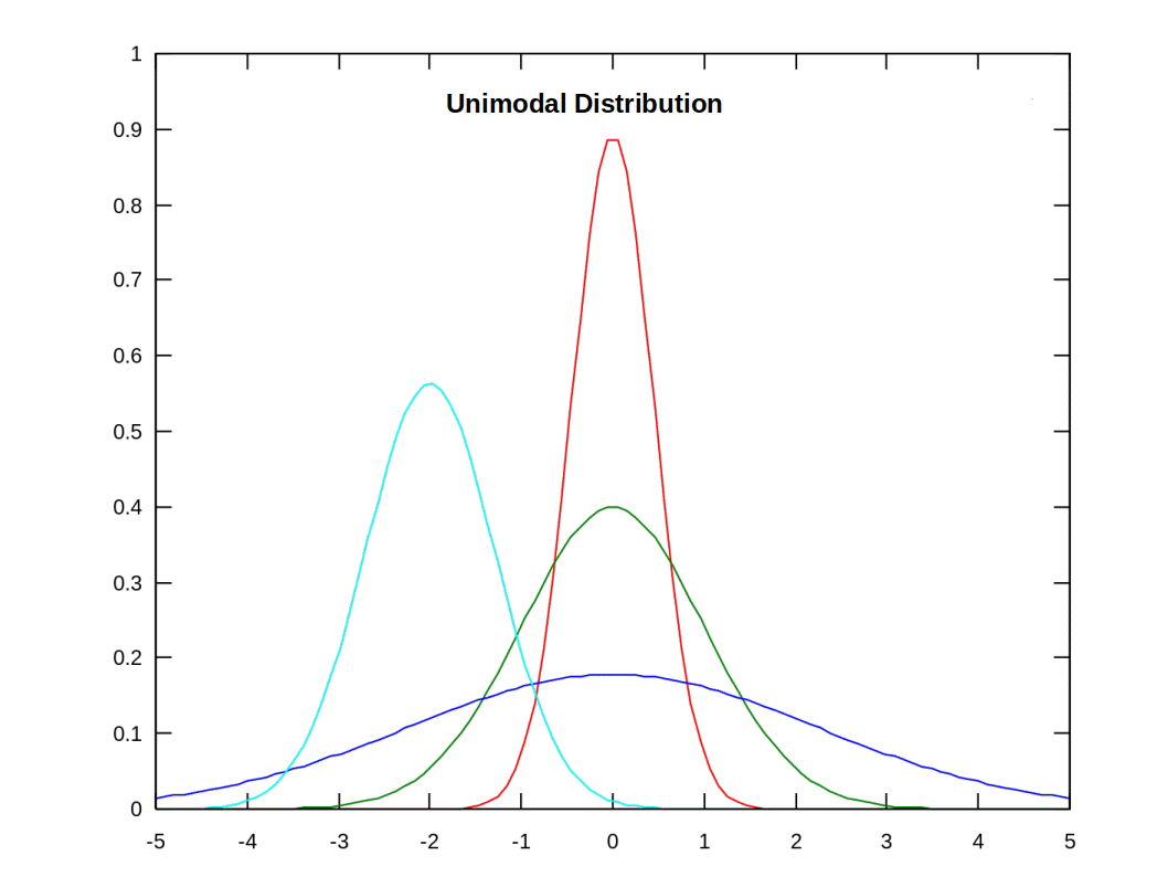 A distribution with two model value is called Bimodal and with more than two is Multimodal.
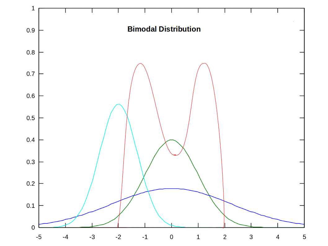 It may so happen that there may be no mode at all in a distribution when no value appears more frequently than any other value. For example, in a series 1, 1, 2, 2, 3, 3, 4, 4, there is no mode.
INDIVIDUAL SERIES
Mode = 3 median – 2 mean
DISCRETE SERIES
X
Frequencies
5
7
10
12
15
15
20
18
25
13
30
10
35
5
40
2
CONTINUOUS SERIES
 L = lower limit of the modal class
X
Frequencies
0 – 5
7
5 – 10
10
10 – 15
12
15 – 20
18
20 – 25
13
25 – 30
8
30 – 35
5
35 – 40
2
X
Frequencies
0 – 5
7
5 – 10
10
10 – 15
12
15 – 20
18
20 – 25
13
25 – 30
8
30 – 35
5
35 – 40
2
X
Frequencies
0 – 9
22
10 – 19
34
20 – 29
53
30 – 39
85
40 – 49
48
50 – 59
26
60 – 69
18
70 – 79
14
X
Frequencies
.5 – 9.5
22
9.5 – 19.5
34
19.5 – 29.5
53
29.5 – 39.5
85
39.5 – 49.5
48
49.5 – 59.5
26
59.5 – 69.5
18
69.5 – 79.5
14
X
Frequencies
Less than 100
40
100 – 200
89
200 – 300
148
300 – 400
64
400 and above
39
X
Frequencies
Less than 100
40
100 – 200
89
200 – 300
148
300 – 400
64
400 and above
39
Value
Frequencies
Less than 60
65
” ” 80
185
” ” 100
270
” ” 120
342
Less than 140
400
Value
Frequencies
40 – 60
65
60 – 80
120
80 – 100
85
100 – 120
72
120 – 140
58
Value
Frequencies
0 – 30
9
30 – 40
8
40 – 50
15
50 – 60
9
60 – 70
3
70 – 90
4
Value
Frequencies
0 – 10
3
10 – 20
3
20 – 30
3
30 – 40
8
40 – 50
15
50 – 60
9
60 – 70
3
70 – 90
4
70 – 80
2
80 – 90
2
LOCATING MODE GRAPHICALLY
X
Frequencies
0 – 100
12
100 – 200
18
200 – 300
27
300 – 400
20
400 – 500
17
500 – 600
6


MERITS OF MODE
DEMERITS OF MODE
Relative Position of Arithmetic Mean, Median and Mode
![]()
0 Comments